The goal of the DasGuptR package is to provide an implementation of Prithwis Das Gupta’s specification of standardization and decomposition of rates, as set out in his 1993 book Standardization and decomposition of rates: A user’s manual.
You can install DasGuptR from here with:
# install.packages("devtools")
devtools::install_github("josiahpjking/DasGuptR")Standardization and decomposition are widely used analytic techniques to adjust for the impact of compositional factors on rates.
Standardization/Adjustment: Shows us what a rate would have been under different scenarios - for example, if there was no difference in the age-structure of the population, or if there was no change in the age-specific rates of the event we are studying.
Decomposition: Gives us the percentage of the difference in rates between two years attributable to each of the factors we have included in the standardization.
In the simplest example, consider a case where the rate is taken as the product of two factors \(\alpha\) and \(\beta\), which we will write as \(R = \alpha\beta\). Throughout Das Gupta’s work, greek letters are used to indicate the different compositional factors, and upper and lower case latin letters are used to denote specific population values of these:
| pop1 | pop2 | |
|---|---|---|
| \(\alpha\) | \(A\) | \(a\) |
| \(\beta\) | \(B\) | \(b\) |
| crude rate | \(AB\) | \(ab\) |
In this simple case, we can standardise across the two populations, calculating \(\alpha\)-standardised rates by replacing \(A\) and \(a\) with \(\frac{a+A}{2}\).
| pop1 | pop2 | |
|---|---|---|
| \(\alpha\) | \(A\) | \(a\) |
| \(\beta\) | \(B\) | \(b\) |
| crude rate, \(R_{crude}\) | \(AB\) | \(ab\) |
| “\(\beta\)-standardised rate”, \(R_{-\alpha}\) | \(A\frac{B+b}{2}\) | \(a\frac{B+b}{2}\) |
| “\(\alpha\)-standardised rate”, \(R_{-\beta}\) | \(\frac{A+a}{2}B\) | \(\frac{A+a}{2}b\) |
These \(\alpha\)-standardised rates can be interpreted as “what the crude rate would look like if \(\alpha\) was held equal” (and analogously for \(\beta\)). In cases involving multiple factors, this can quickly become unwieldy, requiring listing the \(K-1\) factors that are held equal for each standardised rate.1 For this reason, we opt to refer to these rates as, e.g., \(K-\alpha\), where \(K\) is the set of all compositional factors. This is reflected in the table above, where we have used \(R_{crude}\), \(R_{-\alpha}\) and \(R_{-\beta}\) to denote, respectively, the crude rate, the \(K-\alpha\)-standardised rate (or “\(\beta\)-standardised”), and the \(K-\beta\)-standardised (or “\(\alpha\)-standardised”) rate. The \(K-\alpha\)-standardised rate can therefore be interpreted as “what the crude rate would look like if \(\alpha\) changed but all other factors were held equal”.
The difference in the standardised rates is known as a decomposition effect, so named because differences in the crude rates can be decomposed into differences in standardised rates: \(\Delta R_{crude} = \Delta R_{-\alpha} + \Delta R_{-\beta}\). This decomposition allows us to quantify how much of the difference between two crude rates is attributable to differences in \(\alpha\), differences in \(\beta\), and so on. 2
Consider an example of the simple case described above (2 factors, 2 populations).
DasGuptR requires data to be in long format, with columns for each factor, and a single variable denoting the population:
eg.dg <- data.frame(
  pop = c("pop1", "pop2"),
  alpha = c(.6, .3),
  beta = c(.5, .45)
)
eg.dg
#>    pop alpha beta
#> 1 pop1   0.6 0.50
#> 2 pop2   0.3 0.45
In this case, the calculations for the standardised rates can easily be calculated manually:
data.frame(
  pop = c("pop1", "pop2"),
  Rcrude = c(.6 * .5, .3 * .45),
  R_alpha = c(.6, .3) * ((.5 + .45) / 2),
  R_beta = ((.6 + .3) / 2) * c(.5, .45)
)
#>    pop Rcrude R_alpha R_beta
#> 1 pop1  0.300  0.2850 0.2250
#> 2 pop2  0.135  0.1425 0.2025
The workhorse of the DasGuptR package is dgnpop(), which
computes the standardised rates for \(K\) factors across \(N\) populations:
dgnpop(eg.dg, pop = "pop", factors = c("alpha", "beta"))
#>     rate  pop std.set factor
#> 1 0.3000 pop1    <NA>  crude
#> 2 0.1350 pop2    <NA>  crude
#> 3 0.2850 pop1    pop2  alpha
#> 4 0.1425 pop2    pop1  alpha
#> 5 0.2250 pop1    pop2   beta
#> 6 0.2025 pop2    pop1   beta
These can be quickly turned into a wide table in the style of Das
Gupta using dg_table(). When working with just two
populations, this also provides the difference in rates, and expresses
them as the percentage of the crude rate difference:
dgnpop(eg.dg, pop = "pop", factors = c("alpha", "beta")) |>
dg_table()
#> pop1 pop2 diff decomp
#> alpha 0.285 0.1425 -0.1425 86.36
#> beta 0.225 0.2025 -0.0225 13.64
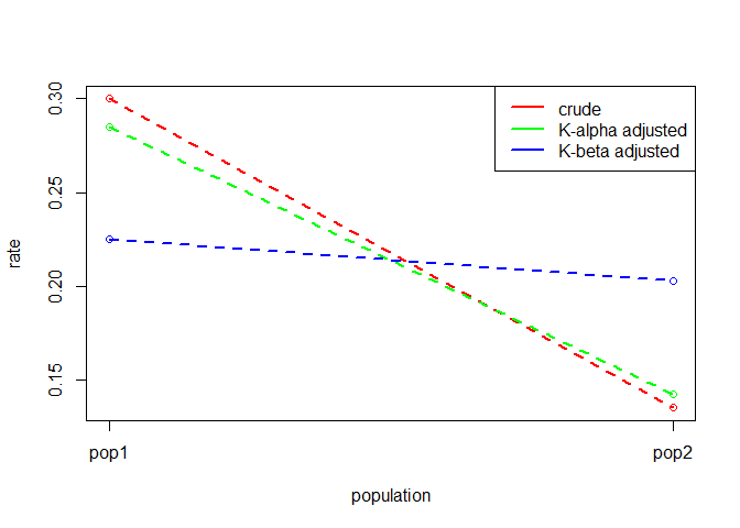
#> crude 0.300 0.1350 -0.1650 100.00In addition to the tabular form, dg_plot() will create a
rough plot of the standardised rates, although this is really only
useful when working with many populations, such as with time series
data.
dgnpop(eg.dg, pop = "pop", factors = c("alpha", "beta")) |>
  dg_plot()
Rates may be composed of many factors, and they may not be calculated as a simple product. Additionally, we may desire to standardise across many populations — such as in a time series — or we may have be interested in how the compositional structure of populations contributes to the differences in these rates.
The full explanation of Das Gupta’s methodology for standardisation and decomposition are explained in full in his 1993 book Standardization and decomposition of rates: A user’s manual
Below are various examples taken from Das Gupta’s 1993 work, following his exposition by building up the number of factors, vectorisation, generalising to different rate functions, compositional structures of populations, and finally extending the process to more than just two populations.
The addition of factors into the make up of a population rate is
handled in dgnpop() by simply adding the variable name into
the factors argument. The default behaviour will take the
rate to be the product of all factors specified.
avg_earnings = total earnings / persons who earnedearner_prop = persons who earned / total
populationeg2.1 <- data.frame(
pop = c("black", "white"),
avg_earnings = c(10930, 16591),
earner_prop = c(.717892, .825974)
)
dgnpop(eg2.1, pop = "pop", factors = c("avg_earnings", "earner_prop")) |>
dg_table()
#> black white diff decomp
#> avg_earnings 8437.228 12807.14 4369.913 74.61
#> earner_prop 9878.553 11365.82 1487.262 25.39
#> crude 7846.560 13703.73 5857.175 100.00birthsw1549 = births x 1000 / women aged 15-49propw1549 = women aged 15-49 / total womenpropw = total women / total populationeg2.2 <- data.frame(
pop = c("austria", "chile"),
birthsw1549 = c(51.78746, 84.90502),
propw1549 = c(.45919, .75756),
propw = c(.52638, .51065)
)
dgnpop(eg2.2, pop = "pop", factors = c("birthsw1549", "propw1549", "propw")) |>
dg_table()
#> austria chile diff decomp
#> birthsw1549 16.31618 26.75021 10.4340333 51.33
#> propw1549 16.25309 26.81394 10.5608476 51.95
#> propw 22.32040 21.65339 -0.6670084 -3.28
#> crude 12.51747 32.84534 20.3278726 100.00birth_preg = non-marital live births x 100 /
non-marital pregnanciespreg_actw = non-marital pregnancies / sexually active
single womenactw_prop = sexually active single women / total single
womenw_prop = total single women / total womeneg2.3 <- data.frame(
pop = c(1971, 1979),
birth_preg = c(25.3, 32.7),
preg_actw = c(.214, .290),
actw_prop = c(.279, .473),
w_prop = c(.949, .986)
)
dgnpop(eg2.3,
pop = "pop",
factors = c("birth_preg", "preg_actw", "actw_prop", "w_prop")
) |>
dg_table()
#> 1971 1979 diff decomp
#> birth_preg 2.355434 3.044375 0.6889411 23.05
#> preg_actw 2.287936 3.100474 0.8125381 27.18
#> actw_prop 1.988818 3.371723 1.3829055 46.26
#> w_prop 2.686817 2.791572 0.1047547 3.50
#> crude 1.433523 4.422663 2.9891394 100.00prop_m = index of proportion marriednoncontr = index of noncontraceptionabort = index of induced abortionlact = index of lactational infecundabilityfecund = total fecundity rateeg2.4 <- data.frame(
pop = c(1970, 1980),
prop_m = c(.58, .72),
noncontr = c(.76, .97),
abort = c(.84, .97),
lact = c(.66, .56),
fecund = c(16.573, 16.158)
)
dgnpop(eg2.4,
pop = "pop",
factors = c("prop_m", "noncontr", "abort", "lact", "fecund")
) |>
dg_table()
#> 1970 1980 diff decomp
#> prop_m 4.519768 5.610746 1.0909785 52.46
#> noncontr 4.450863 5.680707 1.2298438 59.13
#> abort 4.702966 5.430806 0.7278399 35.00
#> lact 5.543146 4.703276 -0.8398707 -40.38
#> fecund 5.152352 5.023334 -0.1290187 -6.20
#> crude 4.050102 6.129875 2.0797729 100.00It is often the case that we have data for each compositional factor on a set of sub-populations, and the crude rates for the population are the aggregated cell-specific rates.
In these cases, dgnpop() requires the user to provide an
appropriate rate function that aggregates up to a summary value for each
population. For instance, in the example below, the cell-specific rates
are calculated as the product of 3 factors, and the population rate is
the sum of the cell-specific rates, so the user would specify
ratefunction = "sum(a*b*c)".
bm = number of births in age-group x 1000 / number of
married women in age-groupmw = number of married women in-age group / total women
in age-groupwp = total women in age-group / total populationeg4.3 <- data.frame(
agegroup = rep(1:7, 2),
pop = rep(c(1970, 1960), e = 7),
bm = c(
488, 452, 338, 156, 63, 22, 3,
393, 407, 369, 274, 184, 90, 16
),
mw = c(
.082, .527, .866, .941, .942, .923, .876,
.122, .622, .903, .930, .916, .873, .800
),
wp = c(
.058, .038, .032, .030, .026, .023, .019,
.043, .041, .036, .032, .026, .020, .018
)
)
dgnpop(eg4.3,
pop = "pop", factors = c("bm", "mw", "wp"),
ratefunction = "sum(bm*mw*wp)"
) |>
dg_table()
#> 1960 1970 diff decomp
#> bm 36.72867 29.44304 -7.285632 62.96
#> mw 34.47028 31.74965 -2.720633 23.51
#> wp 33.83095 32.26577 -1.565181 13.53
#> crude 38.77463 27.20318 -11.571446 100.00Note that for most purposes when working with vector factors, the
population-level rates are what is desired and so users will provide
appropriate rate function. If the rate function provided does
not aggregate up to a summary value, then dgnpop()
will return an array of standardised sub-population rates of the same
length as the number of sub-populations. In order to do this, the user
is also required to specify the variable indicating the sub-population
in id_vars argument.
dgnpop(eg4.3,
  pop = "pop", factors = c("bm", "mw", "wp"),
  id_vars = c("agegroup"),
  ratefunction = "bm*mw*wp"
)
#>          rate  pop std.set factor agegroup
#> 1   2.4892880 1970    1960     bm        1
#> 2  10.2678580 1970    1960     bm        2
#> 3  10.1688427 1970    1960     bm        3
#> 4   4.5237920 1970    1960     bm        4
#> 5   1.5217020 1970    1960     bm        5
#> 6   0.4250290 1970    1960     bm        6
#> 7   0.0465280 1970    1960     bm        7
#> 8   2.0046930 1960    1970     bm        1
#> 9   9.2456155 1960    1970     bm        2
#> ..  ...       ...     ...      ...     ...
#> ..  ...       ...     ...      ...     ...
Returning the array of standardised sub-population rates may be
desired for those looking to calculate category effects as
detailed in
Chevan
& Sutherland 2009 to examine the amount to which a difference in
rates is attributable to differences in specific
sub-populations (see associated vignette with
vignette("category_effects", package="DasGuptR")).
If desired, it is simple retrieve the population rates by aggregating these post-hoc:
library(tidyverse)

dgnpop(eg4.3,
  pop = "pop", factors = c("bm", "mw", "wp"),
  id_vars = c("agegroup"),
  ratefunction = "bm*mw*wp"
) |>
  group_by(pop, factor) |>
  reframe(
    rate = sum(rate)
  )
#> # A tibble: 6 × 3
#>   pop   factor  rate
#>   <chr> <chr>  <dbl>
#> 1 1960  bm      36.7
#> 2 1960  mw      34.5
#> 3 1960  wp      33.8
#> 4 1970  bm      29.4
#> 5 1970  mw      31.7
#> 6 1970  wp      32.3
Equivalently, in the simple case where there is only one variable
indicating a single set of sub-populations (e.g., different age-groups),
then running dgnpop() on data for each sub-population
separately and aggregating up will achieve the same goal:
eg4.3 |>
  nest(data = -agegroup) |>
  mutate(
    dg = map(data, ~ dgnpop(., pop = "pop", factors = c("bm", "mw", "wp")))
  ) |>
  unnest(dg) |>
  group_by(pop, factor) |>
  reframe(
    rate = sum(rate)
  )
#> # A tibble: 8 × 3
#>   pop   factor  rate
#>   <fct> <chr>  <dbl>
#> 1 1960  bm      36.7
#> 2 1960  crude   38.8
#> 3 1960  mw      34.5
#> 4 1960  wp      33.8
#> 5 1970  bm      29.4
#> 6 1970  crude   27.2
#> 7 1970  mw      31.7
#> 8 1970 wp 32.3The ratefunction argument of dgnpop()
essentially allows the user to define a custom rate function. This may
be as simple as \(R = \alpha - \beta\)
(specified as ratefunction = "a-b"):
crude_birth = births x 1000 / total populationcrude_death = deaths x 1000 / total populationeg3.1 <- data.frame(
pop = c(1940, 1960),
crude_birth = c(19.4, 23.7),
crude_death = c(10.8, 9.5)
)
dgnpop(eg3.1,
pop = "pop",
factors = c("crude_birth", "crude_death"),
ratefunction = "crude_birth-crude_death"
) |>
dg_table()
#> 1940 1960 diff decomp
#> crude_birth 9.25 13.55 4.3 76.79
#> crude_death 10.75 12.05 1.3 23.21
#> crude 8.60 14.20 5.6 100.00However, it may be something more complex. For instance, when working
with vector factors, we might define the rate in various ways that
include aggregating over sub-populations in different combinations of
factors (e.g., sum(a*b)/sum(a*b*c)).
The example below shows once such example:
A = number of women in age-group / total womenB = number of unmarried women in age-group / number of
women in age-groupC = births to unmarried women in age-group / number of
unmarried women in age-groupD = births to married women in age-group / married
women in age-groupeg4.4 <- data.frame(
pop = rep(c(1963, 1983), e = 6),
agegroup = c("15-19", "20-24", "25-29", "30-34", "35-39", "40-44"),
A = c(
.200, .163, .146, .154, .168, .169,
.169, .195, .190, .174, .150, .122
),
B = c(
.866, .325, .119, .099, .099, .121,
.931, .563, .311, .216, .199, .191
),
C = c(
.007, .021, .023, .015, .008, .002,
.018, .026, .023, .016, .008, .002
),
D = c(
.454, .326, .195, .107, .051, .015,
.380, .201, .149, .079, .025, .006
)
)
dgnpop(eg4.4,
pop = "pop", factors = c("A", "B", "C", "D"),
id_vars = "agegroup",
ratefunction = "sum(A*B*C) / (sum(A*B*C) + sum(A*(1-B)*D))"
) |>
dg_table()
#> 1963 1983 diff decomp
#> A 0.07770985 0.07150487 -0.00620498 -6.59
#> B 0.04742107 0.09608261 0.04866154 51.64
#> C 0.05924498 0.08630419 0.02705922 28.72
#> D 0.05962676 0.08433604 0.02470928 26.22
#> crude 0.03094957 0.12517462 0.09422505 100.00The ratefunction argument can be given any string that
when parsed and evaluated will return a summary value for a rate. At the
point at which the string is evaluated, each factor (or vector-factor)
is stored in a named list, meaning the function must simply refer to
those factors by name.
It is possible, for instance, to define a custom function in the
user’s environment, and provide a call to that function to the
ratefunction argument of dgnpop():
myratef <- function(a, b, c, d) {
  return(sum(a * b * c) / (sum(a * b * c) + sum(a * (1 - b) * d)))
}

dgnpop(eg4.4,
  pop = "pop", factors = c("A", "B", "C", "D"),
  id_vars = "agegroup",
  ratefunction = "myratef(A,B,C,D)"
) |>
  dg_table()
#>             1963       1983        diff decomp
#> A     0.07770985 0.07150487 -0.00620498  -6.59
#> B     0.04742107 0.09608261  0.04866154  51.64
#> C     0.05924498 0.08630419  0.02705922  28.72
#> D     0.05962676 0.08433604  0.02470928  26.22
#> crude 0.03094957 0.12517462  0.09422505 100.00
The upshot of this is that there is not really any limit to the complexity of the rate function the user wishes to specify. Das Gupta provides one such example in which the rate is obtained iteratively via Newton-Raphson:
Lx = stationary female populationMx = fertility rateeg4.1 <- data.frame(
age_group = c("10-15", "15-20", "20-25", "25-30", "30-35", "35-40", "40-45", "45-50", "50-55"),
pop = rep(c(1965, 1960), e = 9),
Lx = c(
486446, 485454, 483929, 482046, 479522, 475844, 470419, 462351, 450468,
485434, 484410, 492905, 481001, 478485, 474911, 469528, 461368, 449349
),
mx = c(
.00041, .03416, .09584, .07915, .04651, .02283, .00631, .00038, .00000,
.00040, .04335, .12581, .09641, .05504, .02760, .00756, .00045, .00000
)
)
# rate function:
RF4.1 <- function(A, B) {
idx <- seq_len(length(A))
mu0 <- sum(A * B / 100000)
mu1 <- sum((5 * idx + 7.5) * A * B / 100000)
r1 <- log(mu0) * (mu0 / mu1)
while (TRUE) {
Nr1 <- 0
Dr1 <- 0
Nr1 <- Nr1 + sum(exp(-r1 * (5 * idx + 7.5)) * A * (B / 100000))
Dr1 <- Dr1 - sum((5 * idx + 7.5) * exp(-r1 * (5 * idx + 7.5)) * A * (B / 100000))
r2 <- r1 - ((Nr1 - 1) / Dr1)
if (abs(r2 - r1) <= .0000001) {
break
}
r1 <- r2
}
return(r2)
}
# crude rates:
RF4.1(A = eg4.1$Lx[1:9], B = eg4.1$mx[1:9])
#> [1] 0.01213679
RF4.1(A = eg4.1$Lx[10:18], B = eg4.1$mx[10:18])
#> [1] 0.02107187
# decomposition:
dgnpop(eg4.1,
pop = "pop", factors = c("Lx", "mx"),
id_vars = "age_group",
ratefunction = "RF4.1(Lx,mx)"
) |>
dg_table()
#> 1960 1965 diff decomp
#> Lx 0.01670319 0.01649246 -0.0002107251 2.36
#> mx 0.02096000 0.01223564 -0.0087243576 97.64
#> crude 0.02107187 0.01213679 -0.0089350827 100.00Very often, the splitting up of a population into various sub-populations is done because we are interested in that sub-population structure specifically as a compositional factor that could account for differences in crude rates, i.e. separating out how much the crude rate differences are due to differences in the compositional structure of the populations vs differences in the group-specific rates.
To do this, we require data on the sizes (or relative sizes) of each sub-population. The simplest case here would be if we had data on a single set of sub-populations (e.g., age-groups), and had the group-specific rates and group sizes. The crude rates for the population would be simply the sum of all the group-specific rates weighted by the relative size of the group.
In the example below, the relative size of each group is provided as
a percentage in the size column.
size = number in age-group / total populationrate = age-group rateeg5.1 <- data.frame(
age_group = rep(c(
"15-19", "20-24", "25-29", "30-34", "35-39",
"40-44", "45-49", "50-54", "55-59", "60-64",
"65-69", "70-74", "75+"
), 2),
pop = rep(c(1970, 1985), e = 13),
size = c(
12.9, 10.9, 9.5, 8.0, 7.8, 8.4, 8.6, 7.8, 7.0, 5.9, 4.7, 3.6, 4.9,
10.1, 11.2, 11.6, 10.9, 9.4, 7.7, 6.3, 6.0, 6.3, 5.9, 5.1, 4.0, 5.5
),
rate = c(
1.9, 25.8, 45.7, 49.6, 51.2, 51.6, 51.8, 54.9, 58.7, 60.4, 62.8, 66.6, 66.8,
2.2, 24.3, 45.8, 52.5, 56.1, 55.6, 56.0, 57.4, 57.2, 61.2, 63.9, 68.6, 72.2
)
)We can decompose this into the rate-standardised and age-standardised rates in various ways.
eg5.1$age_str <- eg5.1$size / 100

dgnpop(eg5.1,
  pop = "pop", factors = c("age_str", "rate"),
  id_vars = "age_group",
  ratefunction = "sum(age_str*rate)"
) |>
  dg_table()
#>            1970    1985   diff decomp
#> age_str 45.5876 46.8145 1.2269  41.35
#> rate    45.3309 47.0712 1.7403  58.65
#> crude 44.7268 47.6940 2.9672 100.00sum(size) will give us the total population size:dgnpop(eg5.1,
pop = "pop", factors = c("size", "rate"),
id_vars = "age_group",
ratefunction = "sum( (size/sum(size))*rate )"
) |>
dg_table()
#> 1970 1985 diff decomp
#> size 45.5876 46.8145 1.2269 41.35
#> rate 45.3309 47.0712 1.7403 58.65
#> crude 44.7268 47.6940 2.9672 100.00crossclassified argument of
dgnpop().dgnpop(eg5.1,
pop = "pop", factors = c("rate"),
id_vars = "age_group",
crossclassified = "size"
) |>
dg_table()
#> 1970 1985 diff decomp
#> age_group_struct 45.5876 46.8145 1.2269 41.35
#> rate 45.3309 47.0712 1.7403 58.65
#> crude 44.7268 47.6940 2.9672 100.00This latter approach can be extended to situations in which we have cross-classified data - i.e. individual sub-populations are defined by the combination of multiple variables such as age and race.
size = number of people in age-race-grouprate = death rate in age-race-groupeg5.3 <- data.frame(
race = rep(rep(1:2, e = 11), 2),
age = rep(rep(1:11, 2), 2),
pop = rep(c(1985, 1970), e = 22),
size = c(
3041, 11577, 27450, 32711, 35480, 27411, 19555, 19795, 15254, 8022, 2472,
707, 2692, 6473, 6841, 6547, 4352, 3034, 2540, 1749, 804, 236,
2968, 11484, 34614, 30992, 21983, 20314, 20928, 16897, 11339, 5720, 1315,
535, 2162, 6120, 4781, 3096, 2718, 2363, 1767, 1149, 448, 117
),
rate = c(
9.163, 0.462, 0.248, 0.929, 1.084, 1.810, 4.715, 12.187, 27.728, 64.068, 157.570,
17.208, 0.738, 0.328, 1.103, 2.045, 3.724, 8.052, 17.812, 34.128, 68.276, 125.161,
18.469, 0.751, 0.391, 1.146, 1.287, 2.672, 6.636, 15.691, 34.723, 79.763, 176.837,
36.993, 1.352, 0.541, 2.040, 3.523, 6.746, 12.967, 24.471, 45.091, 74.902, 123.205
)
)In these cases, using the sub-population relative sizes as a compositional factor straight off the bat will collapse the two variables that make up the structure of the population:
dgnpop(eg5.3,
  pop = "pop", factors = c("size", "rate"),
  id_vars = c("race", "age"),
  ratefunction = "sum( (size/sum(size))*rate)"
) |>
  dg_table()
#>            1970     1985       diff  decomp
#> size   8.372751 9.914260  1.5415096 -224.64
#> rate  10.257368 8.029643 -2.2277254  324.64
#> crude  9.421833 8.735618 -0.6862158  100.00
Instead, providing the group-specific sizes to the
crossclassified argument will re-express the proportion of
the population in a given cell as a product of factors representing each
of the structural variables. These are then included in the
decomposition:
dgnpop(eg5.3,
  pop = "pop", factors = c("rate"),
  id_vars = c("race", "age"),
  crossclassified = "size"
) |>
  dg_table()
#>                  1970     1985       diff  decomp
#> age_struct   8.385332 9.907067  1.5217347 -221.76
#> race_struct  9.136312 9.156087  0.0197749   -2.88
#> rate        10.257368 8.029643 -2.2277254  324.64
#> crude 9.421833 8.735618 -0.6862158 100.00When standardising across more than two populations, computing the decompositions across all pairs of populations returns N-1 sets of standardised rates, and decompositions between populations that are internally inconsistent (i.e. differences between populations 1 and 2, and 2 and 3, should sum to the difference between 1 and 3).
A = number of women in age-group / total womenB = number of unmarried women in age-group / number of
women in age-groupC = births to unmarried women in age-group / number of
unmarried women in age-groupD = births to married women in age-group / married
women in age-groupeg6.5 <- data.frame(
pop = rep(c(1963, 1968, 1973, 1978, 1983), e = 6),
agegroup = c("15-19", "20-24", "25-29", "30-34", "35-39", "40-44"),
A = c(
.200, .163, .146, .154, .168, .169,
.215, .191, .156, .137, .144, .157,
.218, .203, .175, .144, .127, .133,
.205, .200, .181, .162, .134, .118,
.169, .195, .190, .174, .150, .122
),
B = c(
.866, .325, .119, .099, .099, .121,
.891, .373, .124, .100, .107, .127,
.870, .396, .158, .125, .113, .129,
.900, .484, .243, .176, .155, .168,
.931, .563, .311, .216, .199, .191
),
C = c(
.007, .021, .023, .015, .008, .002,
.010, .023, .023, .015, .008, .002,
.011, .016, .017, .011, .006, .002,
.014, .019, .015, .010, .005, .001,
.018, .026, .023, .016, .008, .002
),
D = c(
.454, .326, .195, .107, .051, .015,
.433, .249, .159, .079, .037, .011,
.314, .181, .133, .063, .023, .006,
.313, .191, .143, .069, .021, .004,
.380, .201, .149, .079, .025, .006
)
)As an illustration, running the standardisation on separate pairs of populations above returns decomposition effects below.
| 1963 v 1968 | 1968 v 1973 | 1963 v 1973 | |
|---|---|---|---|
| A | 0.9773438 | -1.034326 | 0.1688192 |
| B | 5.0282497 | 2.917169 | 7.9721514 |
| C | 7.1177686 | -7.392659 | 1.8923635 |
| D | 9.1479140 | 15.262878 | 21.9910032 |
| Crude | 22.2712761 | 9.753061 | 32.0243373 |
Das Gupta provided a secondary standardisation procedure that takes
sets of pairwise standardised rates and resolves the problems shown
above. When given more than two populations, dgnpop() will
undertake this procedure:
dgnpop(eg6.5,
  pop = "pop", factors = c("A", "B", "C", "D"),
  id_vars = "agegroup",
  ratefunction = "1000*sum(A*B*C) / (sum(A*B*C) + sum(A*(1-B)*D))"
) |>
  dg_table()
#>           1963     1968     1973     1978      1983
#> A     72.77031 74.65254 73.83625 71.36001  64.60057
#> B     53.28255 56.63216 59.52972 79.49763 104.38728
#> C     62.17750 69.61231 60.48031 68.54219  94.17361
#> D     54.83361 64.43823 81.24203 79.60288  74.12756
#> crude 30.94957 53.22084 62.97390 86.88830 125.17462
Because using dg_table() with multiple populations will
not return standardised rates for each population, it will not return
decomposition effects unless only two populations are specified:
dgnpop(eg6.5,
  pop = "pop", factors = c("A", "B", "C", "D"),
  id_vars = "agegroup",
  ratefunction = "1000*sum(A*B*C) / (sum(A*B*C) + sum(A*(1-B)*D))"
) |>
  dg_table(pop1 = 1963, pop2 = 1968)
#>           1963     1968      diff decomp
#> A     72.77031 74.65254  1.882236   8.45
#> B     53.28255 56.63216  3.349606  15.04
#> C     62.17750 69.61231  7.434806  33.38
#> D     54.83361 64.43823  9.604628  43.13
#> crude 30.94957 53.22084 22.271276 100.00
Alternatively, all rate-differences are returned by
dgnpop() if diffs = TRUE, in which case a list
of length 2 is returned, with the first entry providing the standardised
rates, and the second the rate-differences.
dgnpop(eg6.5,
  pop = "pop", factors = c("A", "B", "C", "D"),
  id_vars = "agegroup",
  ratefunction = "1000*sum(A*B*C) / (sum(A*B*C) + sum(A*(1-B)*D))",
  diffs = TRUE
)$diffs
#>           diff  pop diff.calc        std.set factor
#> 1    1.8822361 1963 1963-1968 1973.1978.1983      A
#> 2    1.0659408 1963 1963-1973 1968.1978.1983      A
#> 3   -1.4102979 1963 1963-1978 1968.1973.1983      A
#> 4   -8.1697336 1963 1963-1983 1968.1973.1978      A
#> 5   -0.8162953 1968 1968-1973 1963.1978.1983      A
#> 6   -3.2925340 1968 1968-1978 1963.1973.1983      A
#> ...  ...       ...  ...       ...                 ..
#> ...  ...       ...  ...       ...                 ..
When working with multiple populations in a time series, we can get
quick rough and ready plots of the standardised rates using
dg_plot():
dgnpop(eg6.5,
  pop = "pop", factors = c("A", "B", "C", "D"),
  id_vars = "agegroup",
  ratefunction = "1000*sum(A*B*C) / (sum(A*B*C) + sum(A*(1-B)*D))"
) |>
  dg_plot()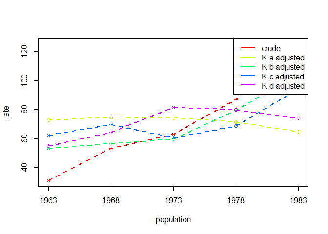
When working with cross-classified data, Das Gupta developed a method of specifying group proportions as set of symmetric proportions indicating the contribution of each structural variable.
Returning to the example above, we can compute these manually for the case of 2 cross-classified variables as so:
eg5.3a <-
  eg5.3 |>
  group_by(pop) |>
  mutate(n_tot = sum(size)) |>
  group_by(pop, age) |>
  mutate(n_age = sum(size)) |>
  group_by(pop, race) |>
  mutate(n_race = sum(size)) |>
  ungroup() |>
  mutate(
    A = ((size / n_race) * (n_age / n_tot))^(1 / 2),
    B = ((size / n_age) * (n_race / n_tot))^(1 / 2),
  )
The product of variables A and B above will
return the individual group proportions:
eg5.3a |>
  mutate(
    AB = A * B,
    prop = size / n_tot
  ) |>
  head()
#> # A tibble: 6 × 12
#>    race   age   pop  size  rate  n_tot n_age n_race      A     B     AB   prop
#>   <int> <int> <dbl> <dbl> <dbl>  <dbl> <dbl>  <dbl>  <dbl> <dbl>  <dbl>  <dbl>
#> 1     1     1  1985  3041 9.16  238743  3748 202768 0.0153 0.830 0.0127 0.0127
#> 2     1     2  1985 11577 0.462 238743 14269 202768 0.0584 0.830 0.0485 0.0485
#> 3     1     3  1985 27450 0.248 238743 33923 202768 0.139  0.829 0.115  0.115
#> 4     1     4  1985 32711 0.929 238743 39552 202768 0.163  0.838 0.137  0.137
#> 5     1     5  1985 35480 1.08  238743 42027 202768 0.176  0.847 0.149  0.149
#> 6     1     6  1985 27411 1.81  238743 31763 202768 0.134  0.856 0.115  0.115
Internally, dgnpop() will do this provided
id_vars and crossclassified are specified as
detailed above. However, should users wish, this intermediary step in
the decomposition can be done using dgcc():
dgcc(eg5.3,
  pop = "pop", id_vars = c("age", "race"),
  crossclassified = "size"
) |>
  head()
#>   race age  pop  size  rate age_struct race_struct
#> 1    1   1 1985  3041 9.163 0.01534415   0.8301237
#> 2    1   2 1985 11577 0.462 0.05841572   0.8301100
#> 3    1   3 1985 27450 0.248 0.13869259   0.8290075
#> 4    1   4 1985 32711 0.929 0.16348055   0.8381024
#> 5    1   5 1985 35480 1.084 0.17550560   0.8467632
#> 6 1 6 1985 27411 1.810 0.13410907 0.8561228birthrate = births per 1000 for age-sex groupthous = population in thousands of age-sex groupdata(uspop)
head(uspop)
#> year agebin thous birthrate
#> 1 1940 10-14 5777 0.7
#> 2 1940 15-19 6145 54.1
#> 3 1940 20-24 5907 135.6
#> 4 1940 25-29 5665 122.8
#> 5 1940 30-34 5192 83.4
#> 6 1940 35-39 4823 46.3
dgo_us <- dgnpop(uspop,
pop = "year", factors = c("birthrate"),
id_vars = "agebin", crossclassified = "thous"
)
dg_plot(dgo_us)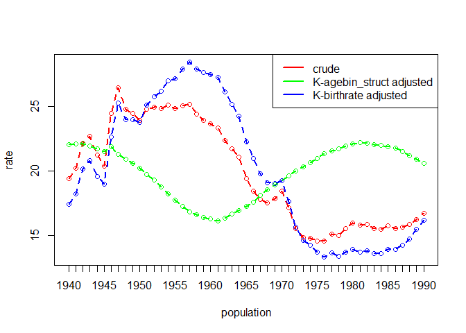
prev_rate = number of reconvicted individuals for
age-sex group / number of offenders in age-sex groupoffenders = number of offenders in age-sex groupconvicted_population = total number of offenders in
populationreconvicted = number of reconvicted individuals for
age-sex groupreconvictions = number of reconvictions for age-sex
groupdata(reconv)
head(reconv)
#> year Sex Age convicted_population offenders reconvicted reconvictions
#> 1 2004 Female 21 to 25 49351 1650 576 1145
#> 2 2004 Female 26 to 30 49351 1268 420 786
#> 3 2004 Female 31 to 40 49351 2238 558 963
#> 4 2004 Female over 40 49351 1198 212 361
#> 5 2004 Female under 21 49351 1488 424 858
#> 6 2004 Male 21 to 25 49351 8941 3285 6330
#> prev_rate
#> 1 0.3490909
#> 2 0.3312303
#> 3 0.2493298
#> 4 0.1769616
#> 5 0.2849462
#> 6 0.3674086
dg_srec <- dgnpop(reconv,
pop = "year", factors = c("prev_rate"),
id_vars = c("Sex", "Age"), crossclassified = "offenders"
)
dg_plot(dg_srec)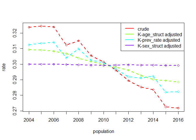
For bootstrapping SEs of decomposition effects as detailed in Wang 2000, see the
associated vignette with
vignette("bootstrap", package="DasGuptR")
For instance, in the case of a rate as the product of four factors \(R = \alpha\beta\gamma\delta\), we get out four sets of standardised rates: the \(\alpha\beta\gamma\)-standardised, \(\beta\gamma\delta\)-standardised, \(\alpha\gamma\delta\)-standardised, and \(\alpha\beta\delta\)-standardised.↩︎
Importantly, the use of “attributable” has a very narrow sense of ‘numerically attributable’, and it is important to stress the lack of any causal interpretation here - different decomposition effects identified by standardization and decomposition may themselves be the products of one (or more) variables not included in the analysis (Das Gupta 1993:4).↩︎