PDQ Functions via Gram Charlier, Edgeworth, and Cornish Fisher Approximations
– Steven E. Pav, shabbychef@gmail.com
This package may be installed from CRAN; the latest development version may be installed via drat, or built from github:
# install via CRAN:
install.packages("PDQutils")

# get latest dev release via drat:
if (require(drat)) {
    drat:::add("shabbychef")
    install.packages("PDQutils")
}

# get snapshot from github (may be buggy)
if (require(devtools)) {
    install_github("shabbychef/PDQutils")
}Approximating the distribution of a random variable via the Gram Charlier, Edgeworth, or Cornish Fisher expansions is most convenient when the random variable can be decomposed as the sum of a small number of independent random variables whose cumulants can be computed. For example, suppose \(Y = \sum_{1 \le i \le k} \sqrt{X_i / \nu_i}\) where the \(X_i\) are independent central chi-square random variables with degrees of freedom \(\nu_1,\nu_2,...,\nu_k\). I will call this a ‘snak’ distribution, for ‘sum of Nakagami’, since each summand follows a Nakagami distribution. We can easily write code that generates variates from this distribution given a vector of the degrees of freedom:
rsnak <- function(n, dfs) {
    samples <- Reduce("+", lapply(dfs, function(k) {
        sqrt(rchisq(n, df = k)/k)
    }))
}
Let’s take one hundred thousand draws from this distribution and see whether it is approximately normal, by performing a q-q plot against a normal distribution.
n.samp <- 1e+05
dfs <- c(8, 15, 4000, 10000)
set.seed(18181)
# now draw from the distribution
rvs <- rsnak(n.samp, dfs)

data <- data.frame(draws = rvs)
mu <- mean(rvs)
sigma <- sd(rvs)
library(ggplot2)
ph <- ggplot(data, aes(sample = draws)) + stat_qq(distribution = function(p) {
    qnorm(p, mean = mu, sd = sigma)
}) + geom_abline(slope = 1, intercept = 0, colour = "red") +
    theme(text = element_text(size = 8)) + labs(title = "Q-Q plot (against normality)")
print(ph)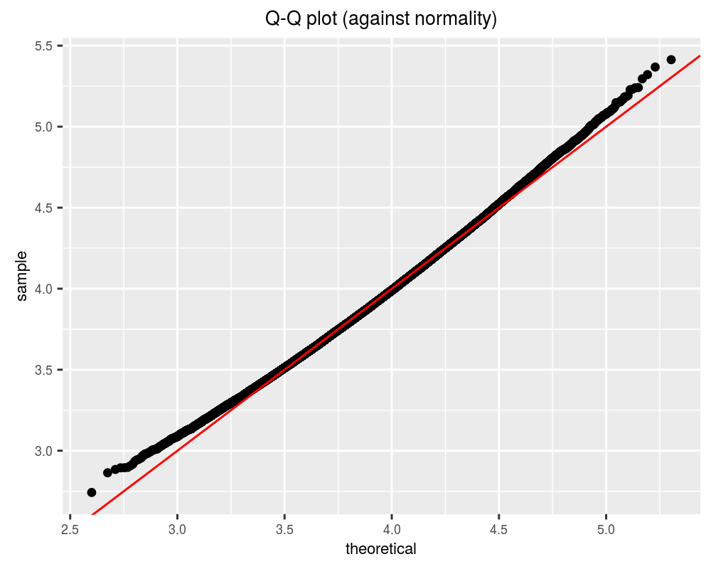
While this is very nearly normal, we can get a better approximation. Using the additivity property of cumulants, we can compute the cumulants of \(Y\) easily if we have the cumulants of the \(X_i\). These in turn can be computed from the raw moments. See wikipedia for the raw moments of the Chi distribution. The following function computes the cumulants:
# for the moment2cumulant function:
library(PDQutils)
# compute the first ord.max raw cumulants of the
# sum of Nakagami variates
snak_cumulants <- function(dfs, ord.max = 10) {
    # first compute the raw moments
    moms <- lapply(dfs, function(k) {
        ords <- 1:ord.max
        moms <- 2^(ords/2) * exp(lgamma((k + ords)/2) -
            lgamma(k/2))
        # we are dividing the chi by sqrt the d.f.
        moms <- moms/(k^(ords/2))
        moms
    })
    # turn moments into cumulants
    cumuls <- lapply(moms, moment2cumulant)
    # sum the cumulants
    tot.cumul <- Reduce("+", cumuls)
    return(tot.cumul)
}
We can now implement the ‘dpq’ functions trivially using the Edgeworth and Cornish Fisher approximations, as follows:
library(PDQutils)

dsnak <- function(x, dfs, ord.max = 6, ...) {
    raw.cumul <- snak_cumulants(dfs, ord.max)
    retval <- dapx_edgeworth(x, raw.cumul, support = c(0,
        Inf), ...)
    return(retval)
}
psnak <- function(q, dfs, ord.max = 6, ...) {
    raw.cumul <- snak_cumulants(dfs, ord.max)
    retval <- papx_edgeworth(q, raw.cumul, support = c(0,
        Inf), ...)
    return(retval)
}
qsnak <- function(p, dfs, ord.max = 10, ...) {
    raw.cumul <- snak_cumulants(dfs, ord.max)
    retval <- qapx_cf(p, raw.cumul, support = c(0,
        Inf), ...)
    return(retval)
}
The density and distribution functions could also have been implemented via the Gram Charlier expansion, although there seems to be little justification for so doing, as the Edgeworth expansion is often a better approximation.
dsnak_2 <- function(x, dfs, ord.max = 10, ...) {
    raw.moment <- cumulant2moment(snak_cumulants(dfs,
        ord.max))
    retval <- dapx_gca(x, raw.moment, support = c(0,
        Inf), ...)
    return(retval)
}
psnak_2 <- function(q, dfs, ord.max = 10, ...) {
    raw.moment <- cumulant2moment(snak_cumulants(dfs,
        ord.max))
    retval <- papx_gca(q, raw.moment, support = c(0,
        Inf), ...)
    return(retval)
}
The q-q plot looks better now:
data <- data.frame(draws = rvs)
library(ggplot2)
ph <- ggplot(data, aes(sample = draws)) + stat_qq(distribution = function(p) {
    qsnak(p, dfs = dfs)
}) + geom_abline(slope = 1, intercept = 0, colour = "red") +
    theme(text = element_text(size = 8)) + labs(title = "Q-Q against qsnak (C-F appx.)")
print(ph)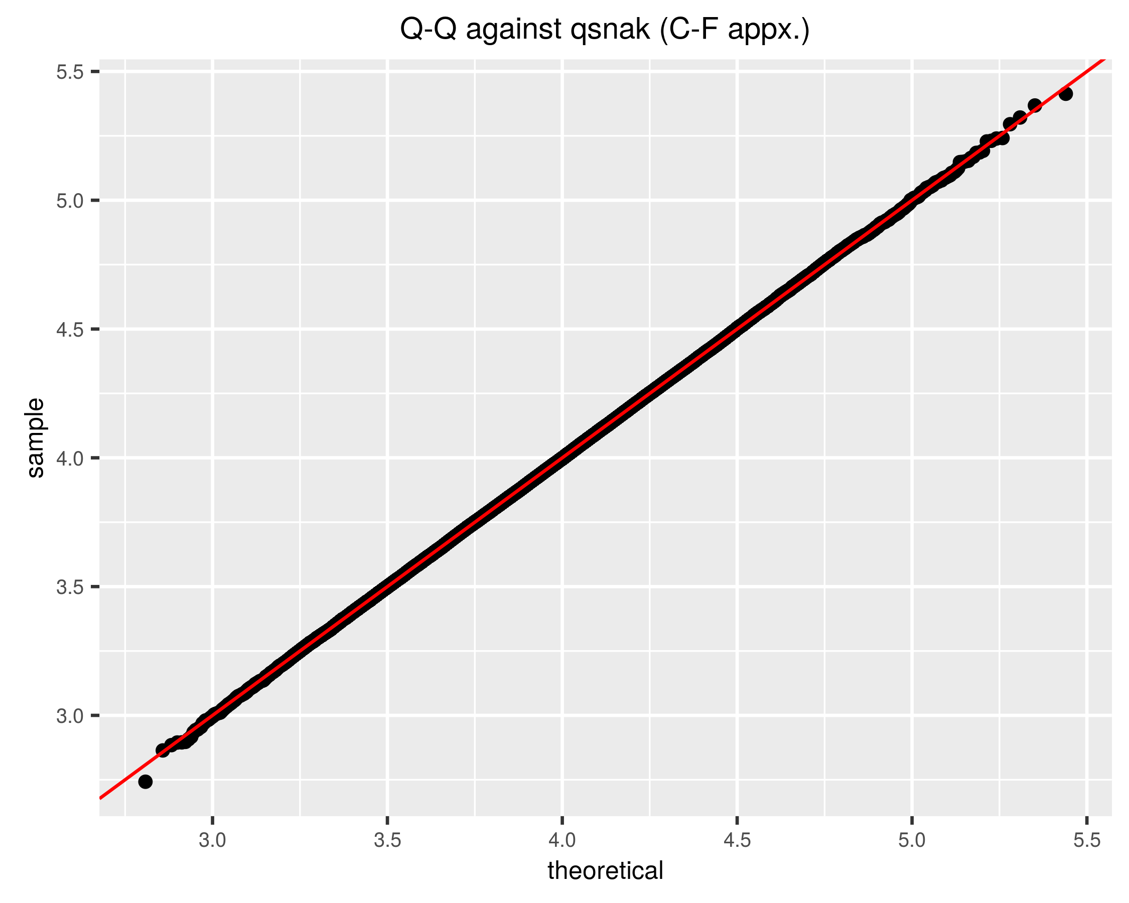
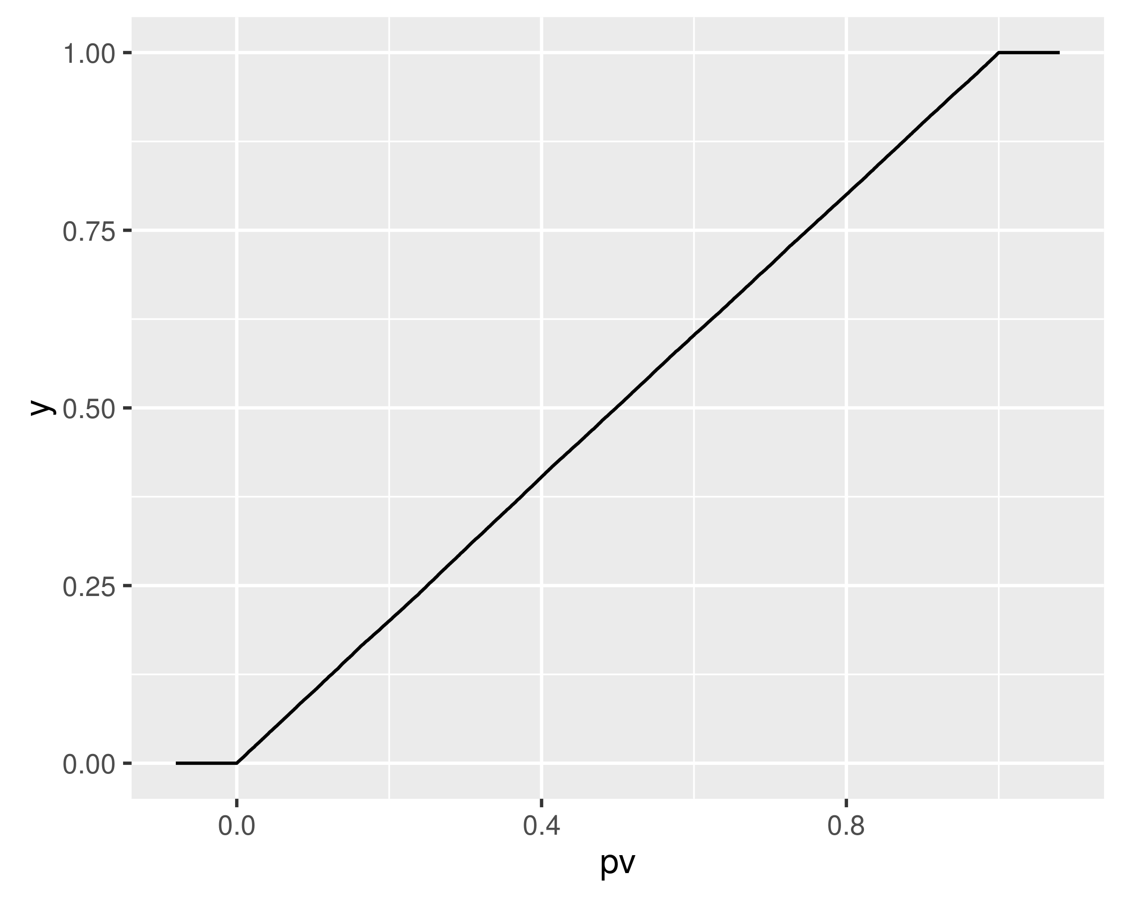
Note that the q-q plot uses the approximate quantile function, qsnak. If we compute the approximate CDF of the random draws, we hope it will be nearly uniform, and indeed it is:
apx.p <- psnak(rvs, dfs = dfs)
if (require(ggplot2)) {
    # qplot(apx.p, stat='ecdf', geom='step')
    ggplot(data.frame(pv = apx.p), aes(x = pv)) + stat_ecdf(geom = "step")
}
Blinnikov and Moessner note that the Gram Charlier expansion will actually diverge for some distributions when more terms in the expansion are considered, behaviour which is not seen for the Edgeworth expansion. We will consider the case of a chi-square distribution with 5 degrees of freedom. The 2 and 6 term Gram Charlier expansions are shown, along with the true value of the PDF, replicating figure 1 of Blinnikov and Moessner:
# compute moments and cumulants:
df <- 5
max.ord <- 20
subords <- 0:(max.ord - 1)
raw.cumulants <- df * (2^subords) * factorial(subords)
raw.moments <- cumulant2moment(raw.cumulants)

# compute the PDF of the rescaled variable:
xvals <- seq(-sqrt(df/2) * 0.99, 6, length.out = 1001)
chivals <- sqrt(2 * df) * xvals + df
pdf.true <- sqrt(2 * df) * dchisq(chivals, df = df)

pdf.gca2 <- sqrt(2 * df) * dapx_gca(chivals, raw.moments = raw.moments[1:2],
    support = c(0, Inf))
pdf.gca6 <- sqrt(2 * df) * dapx_gca(chivals, raw.moments = raw.moments[1:6],
    support = c(0, Inf))

all.pdf <- data.frame(x = xvals, true = pdf.true, gca2 = pdf.gca2,
    gca6 = pdf.gca6)

# plot it by reshaping and ggplot'ing
require(reshape2)
arr.data <- melt(all.pdf, id.vars = "x", variable.name = "pdf",
    value.name = "density")

require(ggplot2)
ph <- ggplot(arr.data, aes(x = x, y = density, group = pdf,
    colour = pdf)) + geom_line()
print(ph)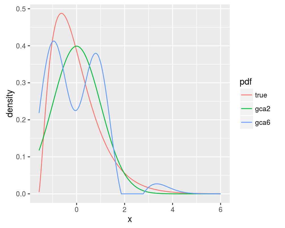
Compare this with the 2 and 4 term Edgeworth expansions, replicating figure 6 of Blinnikov and Moessner:
# compute the PDF of the rescaled variable:
xvals <- seq(-sqrt(df/2) * 0.99, 6, length.out = 1001)
chivals <- sqrt(2 * df) * xvals + df
pdf.true <- sqrt(2 * df) * dchisq(chivals, df = df)

pdf.edgeworth2 <- sqrt(2 * df) * dapx_edgeworth(chivals,
    raw.cumulants = raw.cumulants[1:4], support = c(0,
        Inf))
pdf.edgeworth4 <- sqrt(2 * df) * dapx_edgeworth(chivals,
    raw.cumulants = raw.cumulants[1:6], support = c(0,
        Inf))

all.pdf <- data.frame(x = xvals, true = pdf.true, edgeworth2 = pdf.edgeworth2,
    edgeworth4 = pdf.edgeworth4)

# plot it by reshaping and ggplot'ing
require(reshape2)
arr.data <- melt(all.pdf, id.vars = "x", variable.name = "pdf",
    value.name = "density")

require(ggplot2)
ph <- ggplot(arr.data, aes(x = x, y = density, group = pdf,
    colour = pdf)) + geom_line()
print(ph)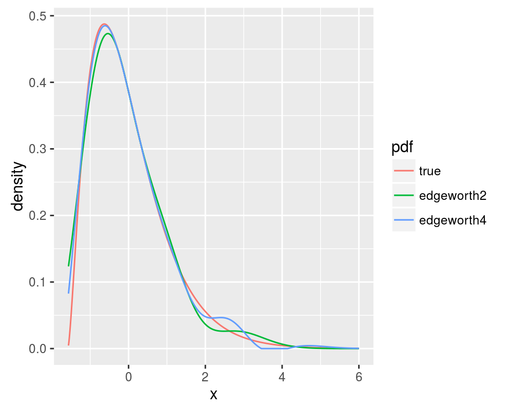
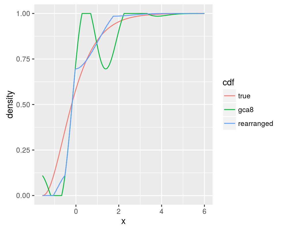
In one of a series of papers, Chernozhukov et. al. demonstrate the use of monotonic rearrangements in Edgeworth and Cornish-Fisher expansions of the CDF and quantile functions, which are, by definition, non-decreasing. It is shown that monotone rearrangement reduces the error of an initial approximation. This is easy enough to code with tools readily available in R. First, let us compute the 8 term Gram Charlier approximation to the CDF of the Chi-square with 5 degrees of freedom. This should display non-monotonicity. Then we compute the monotonic rearrangement:
df <- 5
max.ord <- 20
subords <- 0:(max.ord - 1)
raw.cumulants <- df * (2^subords) * factorial(subords)
raw.moments <- cumulant2moment(raw.cumulants)

# compute the CDF of the rescaled variable:
xvals <- seq(-sqrt(df/2) * 0.99, 6, length.out = 1001)
chivals <- sqrt(2 * df) * xvals + df
cdf.true <- pchisq(chivals, df = df)
cdf.gca8 <- papx_gca(chivals, raw.moments = raw.moments[1:8],
    support = c(0, Inf))

# it is this simple:
require(quantreg)
in.fn <- stepfun(xvals, c(0, cdf.gca8))
out.fn <- rearrange(in.fn)
cdf.rearranged <- out.fn(xvals)

all.cdf <- data.frame(x = xvals, true = cdf.true, gca8 = cdf.gca8,
    rearranged = cdf.rearranged)

# plot it by reshaping and ggplot'ing
require(reshape2)
arr.data <- melt(all.cdf, id.vars = "x", variable.name = "cdf",
    value.name = "density")

require(ggplot2)
ph <- ggplot(arr.data, aes(x = x, y = density, group = cdf,
    colour = cdf)) + geom_line()
print(ph)