Gravitational and magnetic attraction of 3-D vertical rectangular prisms
gravmagsubs is a software package for the R language (R Core Team 2021) for forward modeling of gravity and magnetic anomalies from collections of 3-D right rectangular prisms. The package implements computational approaches developed by (Plouff 1975a, 1975b, 1976) for forward modeling of gravity and magnetic anomalies.
This package is dependent on the following R packages:
Rcpp - Seamless R and C++ Integration (Eddelbuettel and
Francois 2011)
citation("gravmagsubs")##
## To cite gravmagsubs in publications, please use:
##
## Cronkite-Ratcliff, C., Phelps, G., Scheirer, D., 2022, gravmagsubs:
## Gravitational and magnetic attraction of 3-D vertical rectangular
## prisms, U.S. Geological Survey software release, R package, version
## 1.0, https://doi.org/10.5066/P9HBSPRM
##
## A BibTeX entry for LaTeX users is
##
## @Manual{,
## author = {Collin Cronkite-Ratcliff and Geoffrey Phelps and Daniel Scheirer},
## title = {gravmagsubs: Gravitational and magnetic attraction of 3-D vertical rectangular prisms},
## publisher = {U.S. Geological Survey},
## address = {Reston, VA},
## version = {1.0},
## note = {R package},
## institution = {U.S. Geological Survey},
## year = {2022},
## doi = {10.5066/P9HBSPRM},
## url = {https://doi.org/10.5066/P9HBSPRM},
## }It is assumed that users already have installed R (https://www.r-project.org) (R Core Team 2021).
Pandoc (https://pandoc.org) is required to create the package vignettes. Pandoc can be obtained by installing the Rstudio IDE (https://posit.co/), which comes with Pandoc. If you do not install the Rstudio IDE, you will need to install Pandoc individually (https://pandoc.org/installing.html).
Use the remotes package (Csárdi et al. 2022) to install
the package directly from code.usgs.gov. When running
remotes::install_gitlab, you may be asked:
# If you've never installed the "remotes" package:
install.packages("remotes")

#Installing the package from gitlab
remotes::install_gitlab("gmegsc/gravmagsubs",
                        host = "code.usgs.gov",
                        build_opts = c("--no-resave-data",
                                       "--no-manual"),
                        dependencies = TRUE,
                        build_vignettes = TRUE)

These packages have more recent versions available.
It is recommended to update all of them.
Which would you like to update?

1: All
2: CRAN packages only
3: None

Enter one or more numbers, or an empty line to skip updates: 3
Choose “3. None” by typing the number 3, and update all packages after the installation.
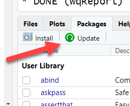
Regularly, it is a good idea to update ALL your packages in R. If using RStudio, this is quite easy, there’s an Update button in the “Packages” tab. This checks CRAN for updates. It is a good idea to click this update regularly.

After installation, in order to use the package, load the package into the R session:
library(gravmagsubs)For help on how to use the package, use the following command to view the documentation for the package:
?gravmagsubsor
help(gravmagsubs)To view the documentation for the functions
rectprismgrav() or rectprismmag():
?rectprismgrav
?rectprismmag
or
help(rectprismgrav)
help(rectprismmag)The gravmagsubs package provides tools for computing the
gravitational and magnetic anomalies generated by 3-D vertical
rectangular prisms at specific observation points. The package consists
of two functions:
rectprismgrav() : Computes the gravitational
attraction of 3-D right rectangular prisms.
rectprismmag() : Computes the magnetic effect of 3-D
right rectangular prisms.
Each function can compute the total anomaly of a series of N prisms at M observation points, returned as a matrix of M rows and 1 column.
Each function also has a logical flag bycell (default
FALSE). If bycell=TRUE, the function returns
the contribution from each individual prism. In this case, the function
will return a matrix of M rows by N columns.
The rectprismgrav() function calculates the gravity
anomaly from a series of 3-D rectangular prisms with vertical sides
using the algorithm of Plouff (1975a).
To calculate the gravity anomaly of a single prism at a single point:
#########################################################
## gravity anomaly of a single prism at a single point ##

# location of the point where the gravity anomaly will be calculated
gravstation <- data.frame(x=0, y=0, z=0)

# the rectangular prism is defined by its six edges (distance in km)
prism1 <- data.frame(xmin=-5, xmax=5,
                     ymin=-5, ymax=5,
                     zmin=-10, zmax=-5)

# density contrast in g/cc
drho <- 0.3

gravanom <- rectprismgrav(gravstation$x, gravstation$y, gravstation$z,
                          prism1$xmin, prism1$xmax,
                          prism1$ymin, prism1$ymax,
                          prism1$zmin, prism1$zmax, drho)

# gravity anomaly (mGal)
print(gravanom)
## [,1]
## [1,] 13.17689To calculate the gravity anomaly at multiple stations along a 2-D cross-section:
#########################################################
## gravity anomaly from a 2-D section                  ##

# gravity station x-axis locations
grav.calc <- data.frame(X = seq(-25, by=.1, length=500))

# density contrast in g/cc
rho <- -0.67

# 2-D section consists of a layered model with density
# contrast extending to 1 km on the left side and 1.5 km
# on the right side
h1 <- 1.5
h2 <- 1

# create the 2-D section, with prisms measuring 1 km
# horizontally and 100 m vertically.
prism.width.h <- 1
prism.width.v <- 0.1
X1 <- seq(-499.5, 499.5, by=prism.width.h)
Z1 <- seq(-3.95, -0.05, by=prism.width.v)
XZr <- expand.grid(xcenter=X1, Y=0, zcenter=Z1)

# define the density contrast as 0 or -0.67 g/cc.
XZr$density <- 0
XZr$density[XZr$zcenter > -h1] <- rho
XZr$density[XZr$zcenter > -(h1+h2) & XZr$xcenter > 0] <- rho

# the y- and z-locations are both zero
grav.calc$Y <- 0
grav.calc$Z <- 0

# Calculate the gravity anomaly.
# Extend the prisms +/-500 km in the Y direction
# to approximate a perfect 2-D model.
grav.calc$Ggms <- rectprismgrav(grav.calc$X, grav.calc$Y, grav.calc$Z,
                                XZr$xcenter - prism.width.h/2,
                                XZr$xcenter + prism.width.h/2,
                                XZr$Y - 500, XZr$Y + 500,
                                XZr$zcenter - prism.width.v/2,
                                XZr$zcenter + prism.width.v/2, XZr$density)

library(ggplot2)

ggplot() +
  geom_line(data = grav.calc, linewidth=2, aes(x = X, y = Ggms)) +
  labs(title = "", x = "Distance [km]", y = "Gravity anomaly (mGal)") +
  theme(panel.background=element_rect(colour="black", fill="white"),
        panel.grid = element_blank(),
        plot.title = element_text(face = "bold",hjust = 0.5, size=16 ),
        aspect.ratio = 1/4)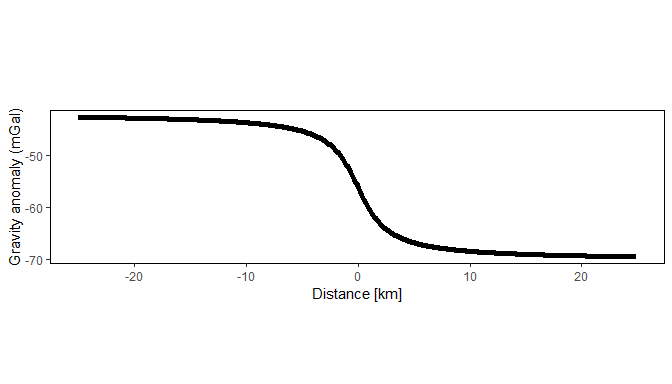
Use the bycell=TRUE option and unit density (1 g/cc) to
obtain the sensitivity matrix.
# Use unit density contrast to obtain sensitivity matrix
XZr$density1 <- 1
XZr.sensmat <- rectprismgrav(grav.calc$X, grav.calc$Y, grav.calc$Z,
                             XZr$xcenter - prism.width.h/2,
                             XZr$xcenter + prism.width.h/2,
                             XZr$Y - 500, XZr$Y + 500,
                             XZr$zcenter - prism.width.v/2,
                             XZr$zcenter + prism.width.v/2, XZr$density1,
                             bycell=TRUE)
Now define two new cross-sections with different density values. The
gravity anomaly of these new cross-sections can be obtained by
multiplying the new density values with the sensitivity matrix, rather
than re-running rectprismgrav().
# Define different density contrast values.
XZr$density2 <- 0
XZr$density2[XZr$density == rho] <- -0.9
XZr$density3 <- 0
XZr$density3[XZr$density == rho] <- -0.4

# Use matrix multiplication to obtain new gravity anomaly.
gravanom.models <- XZr.sensmat %*% as.matrix(XZr[,c("density", "density2", "density3")])

grav.calc$gmod.orig <- gravanom.models[,1]
grav.calc$gmod.low <- gravanom.models[,2]
grav.calc$gmod.high <- gravanom.models[,3]

ggplot() +
  geom_line(data = grav.calc, linewidth=2,
            aes(x = X, y = gmod.low, colour = "-0.9 g/cc")) +
  geom_line(data = grav.calc, linewidth=2,
            aes(x = X, y = gmod.orig, colour = "-0.67 g/cc")) +
  geom_line(data = grav.calc, linewidth=2,
            aes(x = X, y = gmod.high, colour = "-0.4 g/cc")) +
  scale_colour_manual(name="Density contrast", values=c("blue", "black", "red")) +
  labs(title = "", x = "Distance [km]", y = "Gravity anomaly (mGal)") +
  theme(panel.background=element_rect(colour="black", fill="white"),
        legend.key = element_rect(fill = "white"),
        legend.position = "right",
        panel.grid = element_blank(),
        plot.title = element_text(face = "bold", hjust = 0.5, size=16 ),
        aspect.ratio = 1/4)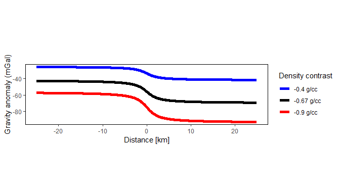
To calculate the gravity anomaly at a 2-D grid of stations located above a 3-D grid of prisms with different density values:
#########################################################
## gravity anomaly from 3-D gridded source model       ##

# first, create an array of stations
xstations <- seq(-5, 5, by=0.1)
ystations <- seq(-5, 5, by=0.1)
D3.stations <- expand.grid(xstations, ystations)
D3.stations$Zstation <- 0
names(D3.stations) <- c("Xstation", "Ystation", "Zstation")

# second, create an array of prisms
width <- 0.1
half.width <- width / 2

xsource <- seq(-2 + half.width, 2 - half.width, by=width)
ysource <- seq(-2 + half.width, 2 - half.width, by=width)
zsource <- seq(-3 + half.width, -1 - half.width, by=width)

D3.source <- expand.grid(xsource, ysource, zsource)
names(D3.source) <- c("xcenter", "ycenter", "zcenter")

# density varies along the y-axis
D3.source$density <- 0.1 * D3.source$ycenter

half.width <- width / 2

D3.gravanom <- rectprismgrav(D3.stations$Xstation,
                             D3.stations$Ystation,
                             D3.stations$Zstation,
                             D3.source$xcenter - half.width,
                             D3.source$xcenter + half.width,
                             D3.source$ycenter - half.width,
                             D3.source$ycenter + half.width,
                             D3.source$zcenter - half.width,
                             D3.source$zcenter + half.width,
                             D3.source$density,
                             bycell=FALSE)

library(scales)

# create data frame
d3.st <- data.frame(x=D3.stations$Xstation, y=D3.stations$Ystation,
                    val1 = D3.gravanom)

# plot with custom color scale
ggplot() +
  geom_raster(data = d3.st, aes(x = x, y = y, fill = val1)) +
  scale_fill_gradientn(
    colours = c("darkblue", "blue", "skyblue", "white", "tomato", "red", "darkred"),
    values = rescale(c(-1.5, 0, 1.5)),
    breaks = seq(-1.5, 1.5, 0.5),
    labels = paste(seq(-1.5, 1.5, 0.5)),
    limits = c(-1.6, 1.6),
    name = "") +
  labs(x = "Easting [km]",
       y = "Northing [km]",
       title = "Gravity anomaly (mGal)") +
  theme(panel.background = element_rect(colour = "black", fill = "white"),
        panel.grid = element_blank(),
        plot.title = element_text(face = "bold", hjust = 0.5, size=16),
        aspect.ratio = 1)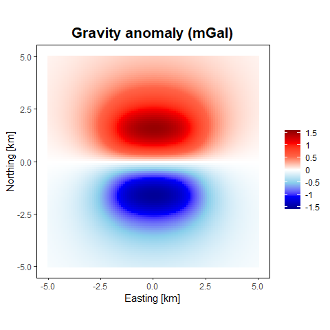
The rectprismmag() function calculates the magnetic
field anomaly from a series of 3-D rectangular prisms with vertical
sides using the algorithm of Plouff (1975b).
To calculate the magnetic anomaly of a single prism at a single point:
#########################################################
## magnetic anomaly of single prism at a single point  ##

# location of the point where the magnetic anomaly will be calculated
magstation <- data.frame(x=-0.3, y=-1.5, z=0)

# the rectangular prism is defined by its six edges (distance in km)
prism1 <- data.frame(xmin=-2, xmax=2,
                     ymin=-2, ymax=2,
                     zmin=-3, zmax=-1)

susc <- 0.015   # susceptiblity (SI)
mstr <- 0       # remanent magnetization (A/m)
mincl <- 0      # remanent inclination (deg)
mdecl <- 0      # remanent declination (deg)
ftotal <- 48800 # Earth's field intensity (nT)
fincl <- 60     # field inclination (deg)
fdecl <- 12     # field declination (deg)

maganom <- rectprismmag(magstation$x, magstation$y, magstation$z,
                        prism1$xmin, prism1$xmax,
                        prism1$ymin, prism1$ymax,
                        prism1$zmin, prism1$zmax, susc,
                        mstr, mincl, mdecl,
                        ftotal, fincl, fdecl)

# magnetic anomaly (nT)
print(maganom)
## [,1]
## [1,] 131.161Calculate the magnetic anomaly at a 2-D grid of stations located above a 3-D grid of prisms. In this example, susceptibility values are generated randomly from a normal distribution with a mean of 0.015 SI units and a standard deviation of 0.001 SI units. No remanent magnetization is present in this example, so the magnetic anomaly is generated entirely from induced magnetization.
#########################################################
## magnetic anomaly from 3-D gridded source model      ##

# first, create an array of stations
xstations <- seq(-5, 5, by=0.1)
ystations <- seq(-5, 5, by=0.1)
D3.stations <- expand.grid(xstations, ystations)
D3.stations$Zstation <- 0
names(D3.stations) <- c("Xstation", "Ystation", "Zstation")

# second, create an array of prisms
width <- 0.1
half.width <- width / 2

xsource <- seq(-2 + half.width, 2 - half.width, by=width)
ysource <- seq(-2 + half.width, 2 - half.width, by=width)
zsource <- seq(-3 + half.width, -1 - half.width, by=width)

D3.source <- expand.grid(xsource, ysource, zsource)
names(D3.source) <- c("xcenter", "ycenter", "zcenter")

# normally distributed, spatially uncorrelated, magnetic susceptibility
set.seed(1)
D3.source$suscnorm <- rnorm(n=length(D3.source[,1]), mean=0.015, sd=0.001)

D3.source$nrmstr <- 0
D3.source$nrmdecl <- 0
D3.source$nrmincl <- 0

# define the ambient field
D3.source$fieldtotal <- 48800
D3.source$fielddecl <- 12
D3.source$fieldincl <- 60

D3.maganomind <- rectprismmag(D3.stations$Xstation,
                              D3.stations$Ystation,
                              D3.stations$Zstation,
                              D3.source$xcenter - half.width,
                              D3.source$xcenter + half.width,
                              D3.source$ycenter - half.width,
                              D3.source$ycenter + half.width,
                              D3.source$zcenter - half.width,
                              D3.source$zcenter + half.width,
                              suscvolsi = D3.source$suscnorm,
                              nrmstr = D3.source$nrmstr,
                              nrmdecl = D3.source$nrmdecl,
                              nrmincl = D3.source$nrmincl,
                              fieldtotal = D3.source$fieldtotal,
                              fielddecl = D3.source$fielddecl,
                              fieldincl = D3.source$fieldincl,
                              bycell=FALSE)

# create data frame
d3.st <- D3.stations
d3.st$val <- D3.maganomind

# plot with custom color scale
ggplot() +
  geom_raster(data = as.data.frame(d3.st),
              aes(x = Xstation, y = Ystation, fill = val)) +
  scale_fill_gradientn(
    colours = c("darkblue", "blue", "lightblue", "white", "pink", "red", "darkred"),
    values = rescale(c(min(d3.st$val), 0, max(d3.st$val))),
    breaks = c(-50, 0, 50, 100),
    labels = paste(c("-50", 0, "50", "100")),
    limits = c(-50, max(d3.st$val)),
    name = "") +
  labs(x = "Distance [km]",
       y = "Distance [km]",
       title = "Induced magnetic anomaly (nT)") +
  theme(panel.background = element_rect(colour="black", fill="white"),
        panel.grid = element_blank(),
        plot.title = element_text(face = "bold", hjust = 0.5, size=16),
        aspect.ratio = 1)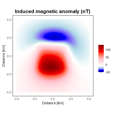
See the current DISCLAIMER