HaploReg (https://pubs.broadinstitute.org/mammals/haploreg/haploreg.php) and RegulomeDB (https://www.regulomedb.org/regulome-search/) are web-based tools that extract biological information such as eQTL, LD, motifs, etc. from large genomic projects such as ENCODE, the 1000 Genomes Project, Roadmap Epigenomics Project and others. This is sometimes called “post stage GWAS” analysis.
The R-package haploR was developed to query those tools (HaploReg and RegulomeDB) directly from R in order to facilitate high-throughput genomic data analysis. Below we provide several examples that show how to work with this package.
Note: you must have a stable Internet connection to use this package.
Contact: ilya.zhbannikov@duke.edu for questions of usage the haploR or any other issues.
This package was inspired by the fact that many web-based post stage GWAS databases do not have Application Programing Interface (API) and, therefore, do not allow users to query them remotedly from R environment. In our research we used HaploReg and RegulomeDB web databases. These very useful web databases show information about linkage disequilibrium of query variants and variants which are in LD with them, expression quantitative trait loci (eQTL), motifs changed and other useful information. However, it is not easy to include this information into streamlined workflow since those tools also not offer API.
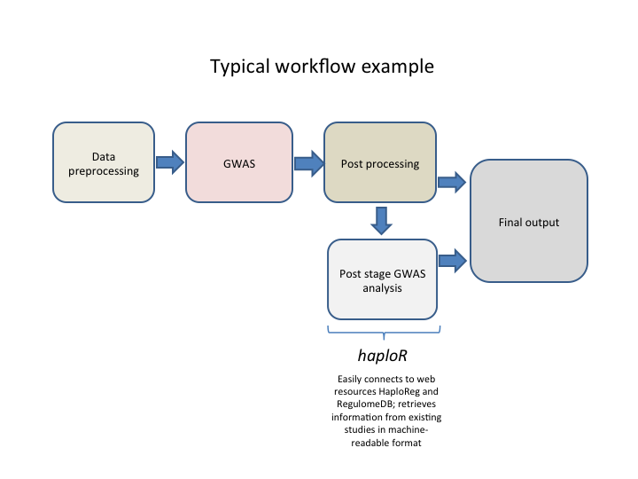
We developed a custom analysis pipeline which prepares data, performs genome-wide association (GWA) analysis and presents results in a user-friendly format. Results include a list of genetic variants (also known as ‘SNP’ or single nucleotide polymorphism), their corresponding p-values, phenotypes (traits) tested and other meta-information such as LD, alternative allele, minor allele frequency, motifs changed, etc. Of course, we could go throught the list of SNPs having genome-wide significant p-values (1e-8) and submit each of those SNPs to HaploReg or RegulomeDB manually, one-by-one, but it is time-consuming process and will not be fully automatic (which ruins one of the pipeline’s paradigms). This is especially difficult if the web site does not offer downloading results.
Therefore, we developed haploR, a user-friendly R package that connects to HaploReg or RegulomeDB from R environment with methods POST and GET and downloads results in a suitable R format. This package siginificantly saved our time in developing reporting system for our internal genomic analysis pipeline and now we would like to present haploR to the research community.
Example of typical analysis workflow is shown below.

In order to install the haploR package, the user must first install R (https://www.r-project.org). After that, haploR can be installed either:
install.packages("haploR", dependencies = TRUE)devtools::install_github("izhbannikov/haplor")haploR depends on the following packages:
Function
queryHaploreg(query = NULL, file = NULL, study = NULL, ldThresh = 0.8,
  ldPop = "EUR", epi = "vanilla", cons = "siphy", genetypes = "gencode",
  url = "https://pubs.broadinstitute.org/mammals/haploreg/haploreg.php",
  timeout = 10, encoding = "UTF-8", verbose = FALSE)
queries HaploReg web-based tool and returns results.
NULL.0.8.AFR (Africa), AMR (America), ASN
(Asia). Default: EUR (Europe).vanilla for ChromHMM (Core 15-state model);
imputed for ChromHMM (25-state model using 12 imputed
marks); methyl for H3K4me1/H3K4me3 peaks;
acetyl for H3K27ac/H3K9ac peaks. Default:
vanilla.gerp for GERP (http://mendel.stanford.edu/SidowLab/downloads/gerp/),
siphy for SiPhy-omega, both for both. Default:
siphy.gencode for Gencode genes; refseq for RefSeq
genes; both for both. Default: gencode.10UTF-8FALSE.A data frame (table) wrapped into a tibble object contains data extracted from HaploReg site. The colums (33 in total at the time of writing this vignette) are specific to HaploReg output. Below we describe the columns:
Number of rows is not constant, at least equal or more than the number of query SNPs, and depends on r2 parameter choosen in a query (default 0.8). This means that the program outputs not only query SNPs, but also those SNPs that have r2 ??? 0.8 with the query SNPs.
library(haploR)
x <- queryHaploreg(query=c("rs10048158","rs4791078"))
x
## # A tibble: 33 x 33
## chr pos_hg38 r2 `D'` is_query_snp rsID ref alt AFR
## <dbl> <dbl> <dbl> <dbl> <dbl> <chr> <chr> <chr> <dbl>
## 1 17 66213160 0.82 0.93 0 rs4790914 C G 0.84
## 2 17 66213422 0.82 0.93 0 rs4791079 T G 0.85
## 3 17 66213896 0.82 0.93 0 rs4791078 A C 0.84
## 4 17 66214285 0.83 0.93 0 rs1971682 G C 0.86
## 5 17 66216124 0.83 0.93 0 rs4366742 T C 0.93
## 6 17 66219453 0.83 0.93 0 rs2215415 G A 0.91
## 7 17 66220526 0.83 0.93 0 rs3744317 G A 0.93
## 8 17 66227121 0.83 0.94 0 rs8178827 C T 0.90
## 9 17 66230111 0.83 0.93 0 rs71160546 GA G 0.87
## 10 17 66231972 0.82 0.99 0 rs11079645 G T 0.88
## # ... with 23 more rows, and 24 more variables: AMR <dbl>, ASN <dbl>,
## # EUR <dbl>, GERP_cons <dbl>, SiPhy_cons <dbl>, Chromatin_States <chr>,
## # Chromatin_States_Imputed <chr>, Chromatin_Marks <chr>, DNAse <chr>,
## # Proteins <chr>, eQTL <chr>, gwas <chr>, grasp <chr>, Motifs <chr>,
## # GENCODE_id <chr>, GENCODE_name <chr>, GENCODE_direction <dbl>,
## # GENCODE_distance <dbl>, RefSeq_id <chr>, RefSeq_name <chr>,
## # RefSeq_direction <dbl>, RefSeq_distance <dbl>,
## # dbSNP_functional_annotation <chr>, query_snp_rsid <chr>Here query is a vector with names of genetic variants.
We then can create a subset from the results, for example, to choose only SNPs with r2 > 0.9:
subset.high.LD <- x[x$r2 > 0.9, c("rsID", "r2", "chr", "pos_hg38", "is_query_snp", "ref", "alt")]
subset.high.LD
## # A tibble: 13 x 7
## rsID r2 chr pos_hg38 is_query_snp ref alt
## <chr> <dbl> <dbl> <dbl> <dbl> <chr> <chr>
## 1 rs10048158 1.00 17 66240200 1 T C
## 2 rs9895261 1.00 17 66244318 0 A G
## 3 rs12603947 0.99 17 66248387 0 T C
## 4 rs7342920 0.99 17 66248527 0 T G
## 5 rs4790914 1.00 17 66213160 0 C G
## 6 rs4791079 1.00 17 66213422 0 T G
## 7 rs4791078 1.00 17 66213896 1 A C
## 8 rs1971682 0.98 17 66214285 0 G C
## 9 rs4366742 0.99 17 66216124 0 T C
## 10 rs2215415 0.99 17 66219453 0 G A
## 11 rs3744317 0.99 17 66220526 0 G A
## 12 rs8178827 0.96 17 66227121 0 C T
## 13 rs71160546 0.94 17 66230111 0 GA GWe can then save the subset.high.LD into an Excel workbook:
require(openxlsx)
write.xlsx(x=subset.high.LD, file="subset.high.LD.xlsx")
This was an example of gathering post-gwas information directly from the online tool. haploR has an additional advantage because it downloads the full information for query retrieved by HaploReg. For example, if you go online and submit these two SNPs to HaploReg (https://pubs.broadinstitute.org/mammals/haploreg/haploreg.php), you will see that some cells of columns “Motifs changed” and “Selected eQTL hits” are hidded (only number of hits are given). haploR retrives this information in a form of a data frame which can be saved into Excel file.
x[, c("Motifs", "rsID")]## # A tibble: 33 x 2
## Motifs
## <chr>
## 1 AP-4_3;Ascl2;E2A_5;Foxa_disc3;HEN1_2;LBP-1_2;NRSF_disc4;NRSF_disc8;NRSF_kno
## 2 Pou5f1_disc1;RFX5_known1;Sox_4;TATA_disc7
## 3 RFX5_known5;Zbtb3
## 4 AP-1_disc1;HEN1_1;Maf_disc2;NR4A_known1;RAR;RXRA_known3;T3R
## 5 Pdx1_2
## 6 AP-1_disc1;HEY1_disc1;TATA_disc2
## 7 .
## 8 ATF3_disc1;LXR_2;SREBP_known4
## 9 Evi-1_3;Irf_disc3;STAT_disc3
## 10 GR_disc4;SZF1-1
## # ... with 23 more rows, and 1 more variables: rsID <chr>x[, c("eQTL", "rsID")]## # A tibble: 33 x 2
## eQTL
## <chr>
## 1 GTEx2015_v6,Heart_Left_Ventricle,PRKCA,3.25964766049438e-10
## 2 GTEx2015_v6,Heart_Left_Ventricle,PRKCA,2.87827072933431e-10;Koopman2014,Hea
## 3 GTEx2015_v6,Heart_Left_Ventricle,PRKCA,2.87827072933431e-10
## 4 GTEx2015_v6,Heart_Left_Ventricle,PRKCA,5.94596439339797e-11
## 5 GTEx2015_v6,Heart_Left_Ventricle,PRKCA,6.83955923561212e-11
## 6 GTEx2015_v6,Heart_Left_Ventricle,PRKCA,6.80544182605399e-11
## 7 GTEx2015_v6,Heart_Left_Ventricle,PRKCA,6.80544182605399e-11;Koopman2014,Hea
## 8 GTEx2015_v6,Heart_Left_Ventricle,PRKCA,2.44658806733437e-10
## 9 GTEx2015_v6,Heart_Left_Ventricle,PRKCA,2.09660151875432e-10
## 10 GTEx2015_v6,Heart_Left_Ventricle,PRKCA,6.18988623085424e-12
## # ... with 23 more rows, and 1 more variables: rsID <chr>If you have a file with your SNPs you would like to analyze, you can supply it as an input as follows:
library(haploR)
x <- queryHaploreg(file=system.file("extdata/snps.txt", package = "haploR"))
x
## # A tibble: 33 x 33
## chr pos_hg38 r2 `D'` is_query_snp rsID ref alt AFR
## <dbl> <dbl> <dbl> <dbl> <dbl> <chr> <chr> <chr> <dbl>
## 1 17 66213160 0.82 0.93 0 rs4790914 C G 0.84
## 2 17 66213422 0.82 0.93 0 rs4791079 T G 0.85
## 3 17 66213896 0.82 0.93 0 rs4791078 A C 0.84
## 4 17 66214285 0.83 0.93 0 rs1971682 G C 0.86
## 5 17 66216124 0.83 0.93 0 rs4366742 T C 0.93
## 6 17 66219453 0.83 0.93 0 rs2215415 G A 0.91
## 7 17 66220526 0.83 0.93 0 rs3744317 G A 0.93
## 8 17 66227121 0.83 0.94 0 rs8178827 C T 0.90
## 9 17 66230111 0.83 0.93 0 rs71160546 GA G 0.87
## 10 17 66231972 0.82 0.99 0 rs11079645 G T 0.88
## # ... with 23 more rows, and 24 more variables: AMR <dbl>, ASN <dbl>,
## # EUR <dbl>, GERP_cons <dbl>, SiPhy_cons <dbl>, Chromatin_States <chr>,
## # Chromatin_States_Imputed <chr>, Chromatin_Marks <chr>, DNAse <chr>,
## # Proteins <chr>, eQTL <chr>, gwas <chr>, grasp <chr>, Motifs <chr>,
## # GENCODE_id <chr>, GENCODE_name <chr>, GENCODE_direction <dbl>,
## # GENCODE_distance <dbl>, RefSeq_id <chr>, RefSeq_name <chr>,
## # RefSeq_direction <dbl>, RefSeq_distance <dbl>,
## # dbSNP_functional_annotation <chr>, query_snp_rsid <chr>File “snps.txt” is a text file which contains one rs-ID per line:
rs10048158
rs4791078Sometimes one would like to explore results from already performed study. In this case you should first explore the existing studies from HaploReg web site (https://pubs.broadinstitute.org/mammals/haploreg/haploreg.php) and then use one of them as an input parameter. See example below:
library(haploR)
# Getting a list of existing studies:
studies <- getStudyList()
# Let us look at the first element:
studies[[1]]
## $name
## [1] "<ce><b2>2-Glycoprotein I (<ce><b2>2-GPI) plasma levels (Athanasiadis G, 2013, 9 SNPs)"
##
## $id
## [1] "1756"# Let us look at the second element:
studies[[2]]## $name
## [1] "5-HTT brain serotonin transporter levels (Liu X, 2011, 1 SNP)"
##
## $id
## [1] "2362"# Query Hploreg to explore results from
# this study:
x <- queryHaploreg(study=studies[[1]])
x## # A tibble: 117 x 33
## chr pos_hg38 r2 `D'` is_query_snp rsID ref alt AFR
## <dbl> <dbl> <dbl> <dbl> <dbl> <chr> <chr> <chr> <dbl>
## 1 11 34524785 0.97 1.00 0 rs836138 C A 0.34
## 2 11 34524788 0.87 0.97 0 rs11032744 C T 0.04
## 3 11 34526877 1.00 1.00 0 rs836137 A G 0.37
## 4 11 34527359 1.00 1.00 0 rs836135 G A 0.36
## 5 11 34527815 1.00 1.00 0 rs704727 T A 0.16
## 6 11 34530979 0.96 0.99 0 rs836133 C T 0.16
## 7 11 34531545 0.90 1.00 0 rs77003093 C T 0.01
## 8 11 34533644 1.00 1.00 1 rs836132 G A 0.16
## 9 11 34534390 1.00 1.00 0 rs836131 C T 0.16
## 10 11 34535548 1.00 1.00 0 rs836130 G T 0.36
## # ... with 107 more rows, and 24 more variables: AMR <dbl>, ASN <dbl>,
## # EUR <dbl>, GERP_cons <dbl>, SiPhy_cons <dbl>, Chromatin_States <chr>,
## # Chromatin_States_Imputed <chr>, Chromatin_Marks <chr>, DNAse <chr>,
## # Proteins <chr>, eQTL <chr>, gwas <chr>, grasp <chr>, Motifs <chr>,
## # GENCODE_id <chr>, GENCODE_name <chr>, GENCODE_direction <dbl>,
## # GENCODE_distance <dbl>, RefSeq_id <chr>, RefSeq_name <chr>,
## # RefSeq_direction <dbl>, RefSeq_distance <dbl>,
## # dbSNP_functional_annotation <chr>, query_snp_rsid <chr>To query RegulomeDB use these 2 functions:
regulomeSummary(query = NULL,
                genomeAssembly = "GRCh37",
                limit=1000,
                timeout=10)
This function queries RegulomeDB https://www.regulomedb.org/regulome-search/ web-based tool and returns results in a named list.
A data frame (table) OR a list with the following items: - guery_coordinates - features - regulome_score - variants - nearby_snps - assembly
library(haploR)
x <- regulomeSummary(c("rs4791078","rs10048158"))
xAccess to LDlink (https://doi.org/10.1093/bioinformatics/btv402) was
temporarily removed from haploR.