Self-reported health, happiness, attitudes, and other statuses or perceptions are often the subject of biases that may come from different sources. For example, the evaluation of an individual’s own health may depend on previous medical diagnoses, functional status, and symptoms and signs of illness; as on well as life-style behaviors, including contextual social, gender, age-specific, linguistic and other cultural factors (Oksuzyan et al. 2019). The hopit package offers versatile functions for analyzing different self-reported ordinal variables, and for helping to estimate their biases. Specifically, the package provides the function to fit a generalized ordered probit model that regresses original self-reported status measures on two sets of independent variables (King et al. 2004; Jurges 2007; Oksuzyan et al. 2019). The first set of variables (e.g., health variables) included in the regression are individual statuses and characteristics that are directly related to the self-reported variable. In the case of self-reported health, these could be chronic conditions, mobility level, difficulties with daily activities, performance on grip strength tests, anthropometric measures, and lifestyle behaviors. The second set of independent variables (threshold variables) is used to model cut-points between adjacent self-reported response categories as functions of individual characteristics, such as gender, age group, education, and country (Oksuzyan et al. 2019). The model helps to adjust for specific socio-demographic and cultural differences in how the continuous latent health is projected onto the ordinal self-rated measure. The fitted model can be used to calculate an individual predicted latent status variable, a latent index, and standardized latent coefficients; and makes it possible to reclassify a categorical status measure that has been adjusted for inter-individual differences in reporting behavior.
Make sure you have the most recent version of R
Run the following code in your R console
hopit packageYou can track (and contribute to) the development of hopit at https://github.com/MaciejDanko/hopit. To install it:
Install the release version of devtools from CRAN with install.packages("devtools").
Make sure you have a working development environment.
Xcode from the Mac App Store.To install the development version of hopit run:
Get started with hopit by checking the vignette or run:
To load the package simply run the following code:
In the example presented below I use healthsurvey, which is a completely artificial data set that is simulated using the distributions of some major health and socio-demographic characteristics. The distributions and the data structure are roughly based on the WAVE1 SHARE database (DOIs: 10.6103/SHARE.w1.600); see Borsch et al. (2013) for technical details about the SHARE database. The structure of healthsurvey for the first six individuals (IDs) is presented below.
data("healthsurvey")
print(t(healthsurvey[1:6,-1]), quote=FALSE, na.print='NA', right=TRUE)
##                                 1       2       3       4         5       6
##  health                 Very good    Good    Good    Good Excellent    Good
##  diabetes                      no      no     yes      no        no      no
##  obese                         no      no      no      no        no      no
##  IADL_problems                 no      no      no      no        no      no
##  hypertension                  no     yes      no      no        no     yes
##  high_cholesterol              no     yes      no      no        no     yes
##  respiratory_problems          no      no      no      no        no     yes
##  heart_attack_or_stroke        no     yes      no      no        no      no
##  poor_mobility                 no      no      no      no        no     yes
##  very_poor_grip                no      no      no      no        no      no
##  depression                    no      no      no     yes        no      no
##  other_diseases               yes     yes      no      no        no     yes
##  sex                          man     man     man     man     woman     man
##  ageclass                     80+   70-79   50-59   60-69       80+     80+
##  education                  prim-   prim-   prim-    sec+     prim-   prim-
##  country                        Y       Y       X       Y         Z       Y
##  csw                      2407.48 1198.12  885.26  772.04   1304.24  917.16
##  psu                           YB      YB      XC      YA        ZB      YD
The first variable on the list (health) is the categorical self-reported health status. This variable is followed by 11 determinants of health, which include information on the presence of chronic diseases and other health conditions. The sex, ageclass, education, and country variables describe the contextual characteristics of individuals. The last group of variables (csw, psu, and ssu) describes the survey design.
The generalized ordered probit models can be fitted using the hopit function. The function takes two kinds of formulas: (1) latent.formula, which models the impact of the latent variables on categorical health; and (2) thresh.formula, which models the thresholds.
One of the crucial steps needed for the proper interpretation of the model results is determining the order of the dependent variable, which must be a factor.
To fit the model, the hopit function is called. Because the order is decreasing (from the best to the worst health state), the hopit parameter decreasing.levels is set to TRUE.
model1 <- hopit(latent.formula = health ~ hypertension +
                             high_cholesterol +
                             heart_attack_or_stroke +
                             poor_mobility +
                             very_poor_grip +
                             depression +
                             respiratory_problems +
                             IADL_problems +
                             obese +
                             diabetes +
                             other_diseases,
               thresh.formula = ~ sex + ageclass,
               decreasing.levels = TRUE,
               data = healthsurvey)
The summary of the fitted model can be created using the summary function.
summary(model1)
##  Formula (latent variables):
##  health ~ hypertension + high_cholesterol + heart_attack_or_stroke +
##      poor_mobility + very_poor_grip + depression + respiratory_problems +
##      IADL_problems + obese + diabetes + other_diseases
##  Formula (threshold variables): ~sex + ageclass
##  Link: probit
##  Number of cases: 10000
##  Response levels: Excellent, Very good, Good, Fair, Poor
##
##  Robust SE were used (sandwich estimator of the variance-covariance matrix).
##
##                            Estimate Std. Error z value Pr(>|z|)
##  hypertensionyes            0.19232    0.02478    7.76  8.4e-15 ***
##  high_cholesterolyes        0.09780    0.02918    3.35  0.00080 ***
##  heart_attack_or_strokeyes  0.34401    0.03183   10.81  < 2e-16 ***
##  poor_mobilityyes           0.72832    0.03564   20.44  < 2e-16 ***
##  very_poor_gripyes          0.49720    0.12299    4.04  5.3e-05 ***
##  depressionyes              0.25323    0.02390   10.59  < 2e-16 ***
##  respiratory_problemsyes    0.36777    0.03337   11.02  < 2e-16 ***
##  IADL_problemsyes           0.61579    0.03637   16.93  < 2e-16 ***
##  obeseyes                   0.18991    0.03295    5.76  8.3e-09 ***
##  diabetesyes                0.33726    0.04010    8.41  < 2e-16 ***
##  other_diseasesyes          0.33533    0.02370   14.15  < 2e-16 ***
##  (L).1|2                   -0.09248    0.03194   -2.90  0.00379 **
##  (L).2|3                   -0.26826    0.03236   -8.29  < 2e-16 ***
##  (L).3|4                    0.07514    0.02905    2.59  0.00968 **
##  (L).4|5                   -0.20346    0.05222   -3.90  9.8e-05 ***
##  (G).sexwoman.1|2           0.02373    0.03015    0.79  0.43111
##  (G).sexwoman.2|3           0.01366    0.03460    0.39  0.69304
##  (G).sexwoman.3|4           0.03661    0.02869    1.28  0.20193
##  (G).sexwoman.4|5           0.11847    0.05039    2.35  0.01872 *
##  (G).ageclass60-69.1|2     -0.01835    0.03383   -0.54  0.58763
##  (G).ageclass60-69.2|3      0.05336    0.04068    1.31  0.18963
##  (G).ageclass60-69.3|4      0.06003    0.03616    1.66  0.09693 .
##  (G).ageclass60-69.4|5      0.16842    0.06492    2.59  0.00949 **
##  (G).ageclass70-79.1|2     -0.32157    0.04391   -7.32  2.4e-13 ***
##  (G).ageclass70-79.2|3      0.17131    0.04774    3.59  0.00033 ***
##  (G).ageclass70-79.3|4      0.19360    0.03777    5.13  3.0e-07 ***
##  (G).ageclass70-79.4|5      0.23235    0.06653    3.49  0.00048 ***
##  (G).ageclass80+.1|2       -0.33134    0.07274   -4.56  5.2e-06 ***
##  (G).ageclass80+.2|3        0.14976    0.07590    1.97  0.04848 *
##  (G).ageclass80+.3|4        0.17851    0.05025    3.55  0.00038 ***
##  (G).ageclass80+.4|5        0.22379    0.07674    2.92  0.00354 **
##  ---
##  Signif. codes:  0 '***' 0.001 '**' 0.01 '*' 0.05 '.' 0.1 ' ' 1
##  Sigma: 1
##  Log-likelihood: -12945.98
##  Deviance: 25891.96
##  AIC: 25953.96
model1 contains 11 dichotomous health variables and two threshold variables. The fitted coefficient includes beta (latent.params, first 11 coefficients in the summary), lambda (thresh.lambda, threshold intercepts, “(L)” prefix in the summary), and gamma (thresh.gamma, parameters related to threshold covariates, “(G)” prefix in the summary). The model coefficients can be accessed directly by the generic coef(model1, aslist = TRUE) function, which has an option to group parameters into a list (aslist = TRUE); or simply by calling model1$coef.ls. The fitted model can be further used to analyze reporting heterogeneity.
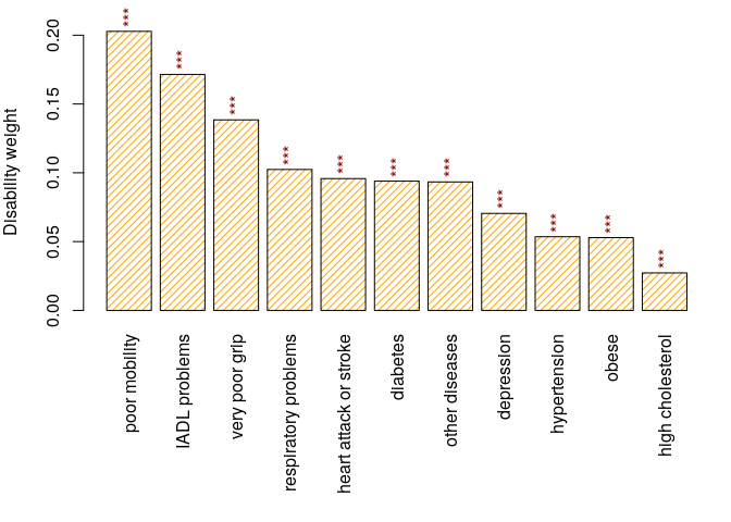
The latent health variables can be directly accessed using model1$coef.ls$latent.params. We can, however, standardize these coefficients using Jürges’ approach (Jurges 2007) in order to obtain so called disability weights. The disability weights are the same for each individual in the modeled population. The standardization is done using the standardizeCoef function.
txtfun <- function(x) gsub('_',' ',substr(x, 1, nchar(x)-3))
sc <- standardizeCoef(model1, namesf = txtfun)
plot(sc)
Figure 1. Disability weights.
The namesf argument is a function or a character vector that is used to rename the coefficients. The exact values of disability weights are stored in sc:
print(sc, show.coef.names=FALSE)
##                         Std. coef
##  hypertension           0.0536
##  high cholesterol       0.0272
##  heart attack or stroke 0.0958
##  poor mobility          0.2028
##  very poor grip         0.1385
##  depression             0.0705
##  respiratory problems   0.1024
##  IADL problems          0.1715
##  obese                  0.0529
##  diabetes               0.0939
##  other diseases         0.0934
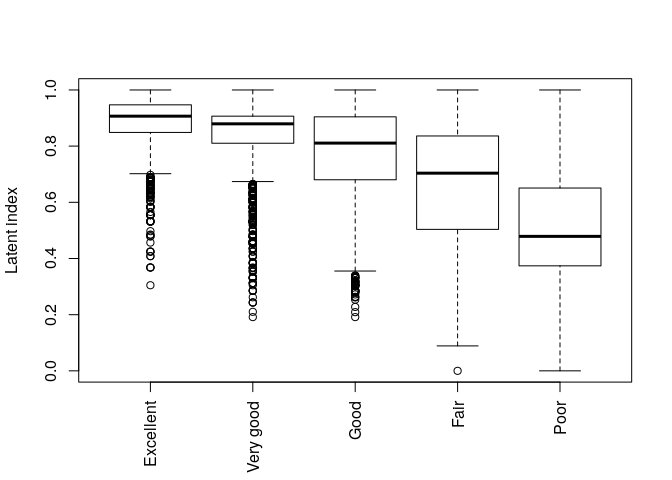
The standardized health status for each individual is called the health index (or the latent index). It is simply calculated using the latentIndex function.

Figure 2. Health index vs. self-reported health.
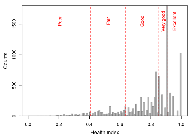
The main aim of the reporting heterogeneity analyses is to determine the cut-points used to calculate the adjusted health status for each individual. The calculation of cut-points is realized using the getCutPoints function.

Figure 3. Health index cut-points for adjusted health levels.
Returned cut-points:
The function also returns adjusted health levels for each individual that are calculated according the Jurges (2007) method:
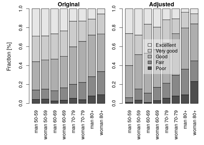
The analysis of health level frequencies is performed using the getLevels function:

Figure 4. Adjusted and original health levels.
The formula describes the grouping variables. It is set to the threshold formula by default, but it can be changed. Here, the country variable is omitted, which means that the age-gender-specific frequencies are calculated for the combined countries. The results are plotted by setting the plotf = TRUE option (Fig. 4). The differences between the original and the adjusted frequencies (%) can be calculated directly using the getLevels output:
round(100*(hl$original - hl$adjusted),2)
##
##                  Poor   Fair   Good Very good Excellent
##    man 50-59     2.93   5.17  -4.08     -6.72      2.70
##    woman 50-59   1.07  -1.16  -5.57      4.80      0.87
##    man 60-69     1.53   0.96  -8.68     -3.96     10.15
##    woman 60-69   0.37  -0.87  -6.48      2.99      3.99
##    man 70-79    -0.10  -1.05  -2.78      2.39      1.53
##    woman 70-79  -3.94  -3.56  -0.66      5.81      2.34
##    man 80+      -1.17  -6.78   0.47      0.23      7.24
##    woman 80+   -13.96   2.67   0.62     10.47      0.21
The package offers the boot_hopit and percentile_CI functions for calculating the confidence intervals for any measure derived from the model using parametric bootstrap methods. In each of the bootstrap repetitions, a new set of model coefficients is drawn from the multivariate normal distribution, taking the originally estimated model coefficients as a mean, and using the model estimated variance-covariance matrix. The drawn coefficients are then used to calculate the measure of interest via a user-defined function. In the example below, I calculate the confidence intervals of the difference between the original and the adjusted frequencies of bad health. The bad health is determined by the presence of “Poor” or “Fair” self-rated health categories.
First, a function to be bootstrapped is defined, which is then used to calculate the mentioned difference:
diff_BadHealth <- function(model) {
  hl <- getLevels(model = model, formula = ~ sex + ageclass, sep = ' ')
  hl$original[,1] + hl$original[,2] - hl$adjusted[,1]- hl$adjusted[,2]
}
The function is used in the boot_hopit function, which also needs to specify a fitted model and the data used to fit model1
The confidence intervals are calculated using the percentile_CI
The same function is used to calculate the difference based on the estimates of the model.
The code below plots the differences and the bootstrapped confidence intervals
pmar <- par('mar'); par(mar = c(7, 5, 0.5, 0.5))
m <- max(abs(est.CI))
pos <- barplot(est.org, names.arg = names(est.org), las = 3,
ylab = 'Original - adjusted differences \nin the prevalences of bad health (%)',
ylim = c(-m, m), density = 20, angle = c(45, -45), col = c('blue', 'orange'))
for (k in seq_along(pos))
   lines(c(pos[k,1],pos[k,1]), est.CI[,k], lwd = 2, col = 2)
abline(h = 0); box(); par(mar = pmar)
Figure 5. Difference between the original and the adjusted prevalences of bad health. The confidence intervals were calculated using the percentile bootstrap method.
The results (Fig. 5) show that men tend to over-report bad health at ages (50,60] and (50,70], whereas women tend to over-report bad health at ages (70,80); and that both sexes tend to under-report bad health at ages (80, 120]. See also Oksuzyan et al. (2019) for similar analyses that were performed using real SHARE data.
This software is an academic project. Any issues and pull requests are welcome. * If hopit is malfunctioning, please report the case by submitting an issue on GitHub. Please see CONTRIBUTING.md for further details.
I thank Anna Oksuzyan, Vladimir M. Shkolnikov, Christian Dudel, Marius Pascariu, Laszlo Nemeth, and Oskar Burger for their comments and suggestions; I thank @alexhanna, the editor of the JOSS journal, and two JOSS peer reviewers @soodoku and @mkearney for their suggestions and corrections. I also thank the Max Planck Institute for Demographic Research for all their support.
The artificially generated data used in the package examples are based on the distributions of some major socio-demographic and health-related characteristics of the WAVE 1 SHARE database. None of the records represent any part of the real data.
The SHARE data collection has been primarily funded by the European Commission through FP5 (QLK6-CT-2001-00360), FP6 (SHARE-I3: RII-CT-2006-062193, COMPARE: CIT5-CT-2005-028857, SHARELIFE: CIT4-CT-2006-028812) and FP7 (SHARE-PREP: N°211909, SHARE-LEAP: N°227822, SHARE M4: N°261982). Additional funding from the German Ministry of Education and Research, the Max Planck Society for the Advancement of Science, the U.S. National Institute on Aging (U01_AG09740-13S2, P01_AG005842, P01_AG08291, P30_AG12815, R21_AG025169, Y1-AG-4553-01, IAG_BSR06-11, OGHA_04-064, HHSN271-201300071C), and various national funding sources is gratefully acknowledged (see www. share-project.org).
Borsch-Supan A, Brandt M, Hunkler C, Kneip T, Korbmacher J, Malter F, Schaan B, Stuck S, and Zuber S. (2013). “Data Resource Profile: The Survey of Health, Ageing and Retirement in Europe (Share).” International Journal of Epidemiology 42 (4): 992–1001. doi: 10.1093/ije/dyt088.
Jurges H,. (2007). “True health vs response styles: exploring cross-country differences in self-reported health.” Health Economics, 16(2), pp. 163-178. doi: 10.1002/hec.1134.
King GC, Murray JL, Salomon JA, and Tandon A. (2004). “Enhancing the Validity and Cross-Cultural Comparability of Measurement in Survey Research.” American Political Science Review 98 (1). Cambridge University Press: 191–207. doi: 10.1017/S000305540400108X.
Oksuzyan A, Danko MJ, Caputo J, Jasilionis D, and Shkolnikov V. (2019). “Is the story about sensitive women and stoical men true? Gender differences in health after adjustment for reporting behavior.” Social Science & Medicine, 228, pp. 41-50. doi: 10.1016/j.socscimed.2019.03.002.