ipd is an open-source R software package
for the downstream modeling of an outcome and its associated features
where a potentially sizable portion of the outcome data has been imputed
by an artificial intelligence or machine learning (AI/ML) prediction
algorithm. The package implements several recent proposed methods for
inference on predicted data (IPD) with a single, user-friendly wrapper
function, ipd. The package also provides custom
print, summary, tidy,
glance, and augment methods to facilitate easy
model inspection.
Using predictions from pre-trained algorithms as outcomes in downstream statistical analyses can lead to biased estimates and misleading conclusions. The statistical challenges encountered when drawing inference on predicted data (IPD) include:
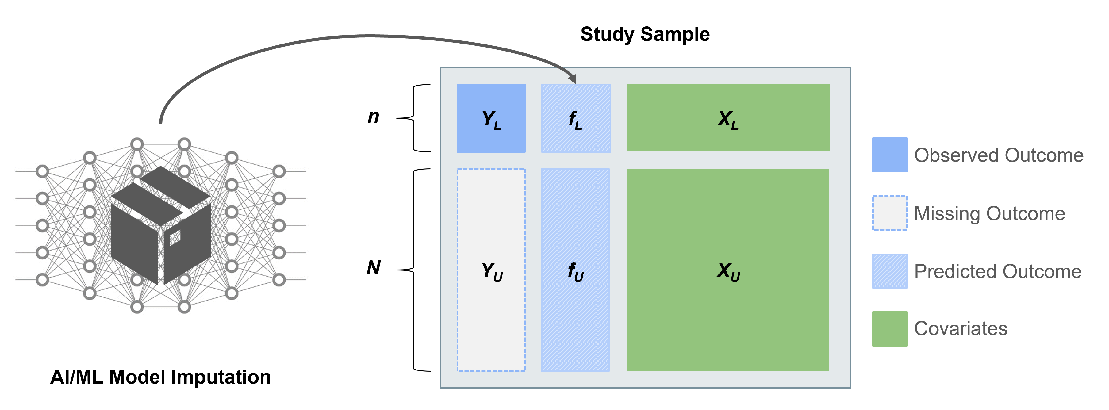
Several works have proposed methods for IPD, including post-prediction inference (PostPI) by Wang et al., 2020, prediction-powered inference (PPI) and PPI++ by Angelopoulos et al., 2023a and Angelopoulos et al., 2023b, and post-prediction adaptive inference (PSPA) by Miao et al., 2023. Each method was developed to perform inference on a quantity such as the outcome mean or quantile, or a regression coefficient, when we have:

We can use these methods for IPD to obtain corrected estimates and standard errors by using the predicted outcomes and unlabeled features to augment the labeled subset of the data.
To enable researchers and practitioners interested in these
state-of-the-art methods, we have developed the ipd package
in R to implement these methods under the umbrella of IPD.
This README provides an overview of the package, including installation
instructions, basic usage examples, and links to further documentation.
The examples show how to generate data, fit models, and use custom
methods provided by the package.
To install the development version of ipd from GitHub, you can use the
devtools package:
#-- Install devtools if it is not already installed

install.packages("devtools")

#-- Install the ipd package from GitHub

devtools::install_github("ipd-tools/ipd")We provide a simple example to demonstrate the basic use of the
functions included in the ipd package.
You can generate synthetic datasets for different types of regression
models using the provided simdat function by specifying the
sizes of the datasets, the effect size, residual variance, and the type
of model. The function currently supports “mean”, “quantile”, “ols”,
“logistic”, and “poisson” models. The simdat function
generate a data.frame with three subsets: (1) an independent “training”
set with additional observations used to fit a prediction model, and
“labeled” and “unlabeled” sets which contain the observed and predicted
outcomes and the simulated features of interest.
#-- Load the ipd Library

library(ipd)

#-- Generate Example Data for Linear Regression

set.seed(123)

n <- c(10000, 500, 1000)

dat <- simdat(n = n, effect = 1, sigma_Y = 4, model = "ols")

#-- Print First 6 Rows of Training, Labeled, and Unlabeled Subsets

options(digits=2)

head(dat[dat$set_label == "training",])
#>       X1    X2    X3     X4     Y  f set_label
#> 1 -0.560 -0.56  0.82 -0.356 -0.15 NA  training
#> 2 -0.230  0.13 -1.54  0.040 -4.49 NA  training
#> 3  1.559  1.82 -0.59  1.152 -1.08 NA  training
#> 4  0.071  0.16 -0.18  1.485 -3.67 NA  training
#> 5  0.129 -0.72 -0.71  0.634  2.19 NA  training
#> 6  1.715  0.58 -0.54 -0.037 -1.42 NA  training

head(dat[dat$set_label == "labeled",])
#>          X1      X2    X3    X4     Y     f set_label
#> 10001  2.37 -1.8984  0.20 -0.17  1.40  3.24   labeled
#> 10002 -0.17  1.7428  0.26 -2.05  3.56  1.03   labeled
#> 10003  0.93 -1.0947  0.76  1.25 -3.66  2.37   labeled
#> 10004 -0.57  0.1757  0.32  0.65 -0.56  0.58   labeled
#> 10005  0.23  2.0620 -1.35  1.46 -0.82 -0.15   labeled
#> 10006  1.13 -0.0028  0.23 -0.24  7.30  2.16   labeled

head(dat[dat$set_label == "unlabeled",])
#>          X1     X2    X3    X4    Y     f set_label
#> 10501  0.99 -3.280 -0.39  0.97  8.4  1.25 unlabeled
#> 10502 -0.66  0.142 -1.36 -0.22 -7.2 -1.08 unlabeled
#> 10503  0.58 -1.368 -1.73  0.15  5.6 -0.31 unlabeled
#> 10504 -0.14 -0.728  0.26 -0.23 -4.2  0.91 unlabeled
#> 10505 -0.17 -0.068 -1.10  0.58  2.2 -0.39 unlabeled
#> 10506  0.58  0.514 -0.69  0.97 -1.2  0.76 unlabeled
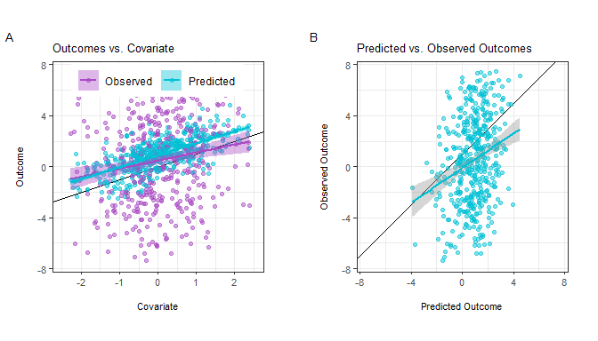
The simdat function provides observed and unobserved
outcomes for both the labeled and unlabeled datasets, though in practice
the observed outcomes are not in the unlabeled set. We can visualize the
relationships between these variables:

We can see that:
We compare two non-IPD approaches to analyzing the data to methods
included in the ipd package. A summary comparison is
provided in the table below, followed by the specific calls for each
method:
#>                    Estimate Std.Error
#> Naive                  0.98      0.03
#> Classic                1.10      0.19
#> PostPI (Bootstrap)     1.16      0.18
#> PostPI (Analytic)      1.15      0.18
#> PPI++                  1.12      0.19
#> PSPA                   1.12      0.19
We can see that the IPD methods have similar estimates and standard errors, while the ‘naive’ method has a different estimate and standard errors that are too small.
#--- Fit the Naive Regression

lm(f ~ X1, data = dat[dat$set_label == "unlabeled",]) |>

  summary()
#>
#> Call:
#> lm(formula = f ~ X1, data = dat[dat$set_label == "unlabeled",
#>     ])
#>
#> Residuals:
#>     Min      1Q  Median      3Q     Max
#> -2.5426 -0.6138 -0.0153  0.6345  2.8907
#>
#> Coefficients:
#>             Estimate Std. Error t value Pr(>|t|)
#> (Intercept)   0.8391     0.0297    28.3   <2e-16 ***
#> X1            0.9848     0.0296    33.3   <2e-16 ***
#> ---
#> Signif. codes:  0 '***' 0.001 '**' 0.01 '*' 0.05 '.' 0.1 ' ' 1
#>
#> Residual standard error: 0.94 on 998 degrees of freedom
#> Multiple R-squared:  0.527,  Adjusted R-squared:  0.526
#> F-statistic: 1.11e+03 on 1 and 998 DF, p-value: <2e-16#--- Fit the Classic Regression
lm(Y ~ X1, data = dat[dat$set_label == "labeled",]) |>
summary()
#>
#> Call:
#> lm(formula = Y ~ X1, data = dat[dat$set_label == "labeled", ])
#>
#> Residuals:
#> Min 1Q Median 3Q Max
#> -15.262 -2.828 -0.094 2.821 11.685
#>
#> Coefficients:
#> Estimate Std. Error t value Pr(>|t|)
#> (Intercept) 0.908 0.187 4.86 1.6e-06 ***
#> X1 1.097 0.192 5.71 1.9e-08 ***
#> ---
#> Signif. codes: 0 '***' 0.001 '**' 0.01 '*' 0.05 '.' 0.1 ' ' 1
#>
#> Residual standard error: 4.2 on 498 degrees of freedom
#> Multiple R-squared: 0.0614, Adjusted R-squared: 0.0596
#> F-statistic: 32.6 on 1 and 498 DF, p-value: 1.95e-08You can fit the various IPD methods to your data and obtain summaries
using the provided wrapper function, ipd():
#-- Specify the Formula

formula <- Y - f ~ X1

#-- Fit the PostPI Bootstrap Correction

nboot <- 200

ipd::ipd(formula,

  method = "postpi_boot", model = "ols", data = dat, label = "set_label",

  nboot = nboot) |>

  summary()
#>
#> Call:
#>  Y - f ~ X1
#>
#> Method: postpi_boot
#> Model: ols
#> Intercept: Yes
#>
#> Coefficients:
#>             Estimate Std.Error Lower.CI Upper.CI
#> (Intercept)    0.866     0.183    0.507     1.22
#> X1 1.164 0.183 0.806 1.52#-- Fit the PostPI Analytic Correction
ipd::ipd(formula,
method = "postpi_analytic", model = "ols", data = dat, label = "set_label") |>
summary()
#>
#> Call:
#> Y - f ~ X1
#>
#> Method: postpi_analytic
#> Model: ols
#> Intercept: Yes
#>
#> Coefficients:
#> Estimate Std.Error Lower.CI Upper.CI
#> (Intercept) 0.865 0.183 0.505 1.22
#> X1 1.145 0.182 0.788 1.50#-- Fit the PPI Correction
ipd::ipd(formula,
method = "ppi", model = "ols", data = dat, label = "set_label") |>
summary()
#>
#> Call:
#> Y - f ~ X1
#>
#> Method: ppi
#> Model: ols
#> Intercept: Yes
#>
#> Coefficients:
#> Estimate Std.Error Lower.CI Upper.CI
#> (Intercept) 0.871 0.182 0.514 1.23
#> X1 1.122 0.195 0.740 1.50#-- Fit the PPI++ Correction
ipd::ipd(formula,
method = "ppi_plusplus", model = "ols", data = dat, label = "set_label") |>
summary()
#>
#> Call:
#> Y - f ~ X1
#>
#> Method: ppi_plusplus
#> Model: ols
#> Intercept: Yes
#>
#> Coefficients:
#> Estimate Std.Error Lower.CI Upper.CI
#> (Intercept) 0.881 0.182 0.524 1.24
#> X1 1.116 0.187 0.750 1.48#-- Fit the PSPA Correction
ipd::ipd(formula,
method = "pspa", model = "ols", data = dat, label = "set_label") |>
summary()
#>
#> Call:
#> Y - f ~ X1
#>
#> Method: pspa
#> Model: ols
#> Intercept: Yes
#>
#> Coefficients:
#> Estimate Std.Error Lower.CI Upper.CI
#> (Intercept) 0.881 0.182 0.524 1.24
#> X1 1.109 0.187 0.743 1.47The package also provides custom print,
summary, tidy, glance, and
augment methods to facilitate easy model inspection:
#-- Fit the PostPI Bootstrap Correction

nboot <- 200

fit_postpi <- ipd::ipd(formula,

  method = "postpi_boot", model = "ols", data = dat, label = "set_label",

  nboot = nboot)

#-- Print the Model

print(fit_postpi)
#>
#> Call:
#>  Y - f ~ X1
#>
#> Coefficients:
#> (Intercept)          X1
#>        0.86        1.15

#-- Summarize the Model

summ_fit_postpi <- summary(fit_postpi)

#-- Print the Model Summary

print(summ_fit_postpi)
#>
#> Call:
#>  Y - f ~ X1
#>
#> Method: postpi_boot
#> Model: ols
#> Intercept: Yes
#>
#> Coefficients:
#>             Estimate Std.Error Lower.CI Upper.CI
#> (Intercept)    0.860     0.183    0.502     1.22
#> X1             1.148     0.182    0.790     1.50

#-- Tidy the Model Output

tidy(fit_postpi)
#>                    term estimate std.error conf.low conf.high
#> (Intercept) (Intercept)     0.86      0.18     0.50       1.2
#> X1                   X1     1.15      0.18     0.79       1.5

#-- Get a One-Row Summary of the Model

glance(fit_postpi)
#>        method model include_intercept nobs_labeled nobs_unlabeled       call
#> 1 postpi_boot   ols              TRUE          500           1000 Y - f ~ X1

#-- Augment the Original Data with Fitted Values and Residuals

augmented_df <- augment(fit_postpi)

head(augmented_df)
#>          X1     X2    X3    X4    Y     f set_label .fitted .resid
#> 10501  0.99 -3.280 -0.39  0.97  8.4  1.25 unlabeled   1.992    6.5
#> 10502 -0.66  0.142 -1.36 -0.22 -7.2 -1.08 unlabeled   0.099   -7.3
#> 10503  0.58 -1.368 -1.73  0.15  5.6 -0.31 unlabeled   1.522    4.1
#> 10504 -0.14 -0.728  0.26 -0.23 -4.2  0.91 unlabeled   0.702   -4.9
#> 10505 -0.17 -0.068 -1.10  0.58  2.2 -0.39 unlabeled   0.667    1.5
#> 10506 0.58 0.514 -0.69 0.97 -1.2 0.76 unlabeled 1.521 -2.7For additional details, we provide more use cases and examples in the package vignette:
vignette("ipd")For questions, comments, or any other feedback, please contact the developers (ssalerno@fredhutch.org).
Contributions are welcome! Please open an issue or submit a pull request on GitHub. The following method/model combinations are currently implemented:
| Method | Mean Estimation | Quantile Estimation | Linear Regression | Logistic Regression | Poisson Regression | Multiclass Regression |
|---|---|---|---|---|---|---|
| PostPI | :x: | :x: | :white_check_mark: | :white_check_mark: | :x: | :x: |
| PPI | :white_check_mark: | :white_check_mark: | :white_check_mark: | :white_check_mark: | :x: | :x: |
| PPI++ | :white_check_mark: | :white_check_mark: | :white_check_mark: | :white_check_mark: | :x: | :x: |
| PSPA | :white_check_mark: | :white_check_mark: | :white_check_mark: | :white_check_mark: | :white_check_mark: | :x: |
| PSPS | :x: | :x: | :x: | :x: | :x: | :x: |
| PDC | :x: | :x: | :x: | :x: | :x: | :x: |
| Cross-PPI | :x: | :x: | :x: | :x: | :x: | :x: |
| PPBoot | :x: | :x: | :x: | :x: | :x: | :x: |
| DSL | :x: | :x: | :x: | :x: | :x: | :x: |
This package is licensed under the MIT License.