
slca provides comprehensive tools for the implementation
of Structural Latent Class Models (SLCM), including Latent Transition
Analysis (LTA; Linda M. Collins and Stephanie T. Lanza, 2009) doi:10.1002/9780470567333, Latent Class Profile Analysis
(LCPA; Hwan Chung et al., 2010) doi:10.1111/j.1467-985x.2010.00674.x, and Joint Latent
Class Analysis (JLCA; Saebom Jeon et al., 2017) doi:10.1080/10705511.2017.1340844, and any other
extended models involving multiple latent class variables.
You can install the released version of slca from CRAN with:
install.packages("slca")And the development version from GitHub with:
# install.packages("devtools")
devtools::install_github("kim0sun/slca")The function serves as the starting point for model specification.
slca(x, ..., constraints = NULL)This primary function is crucial for forming the foundational structure of your analysis, enabling a deep understanding of the intricate latent structures within your dataset. The syntax is organized into two main segments: the measurement model specification and the structural model specification. This logical arrangement enhances the clarity and efficacy of the model development process.
Here, you delve into the heart of your model by defining latent class
variables. These are essentially unobserved variables inferred from
manifest indicators (observable variables). Each latent class variable
is represented alongside its number of classes, denoted in either
parentheses or brackets. For instance, you might define three classes
for latent class variable L1 as L1(3).
Following syntax describes three latent class variables with three
classes each measured by x, y,
z.
L1(3) ~ x1 + x2 + x3
L2[3] ~ y1 + y2 + y3
L3(3) ~ z1 + z2 + z3
This part focuses on establishing relationships between different
latent class variables. For example, L1 ~ L2 indicates a
relationship where L1 have impact on or related to
L2, as shown below:
L1 ~ L2
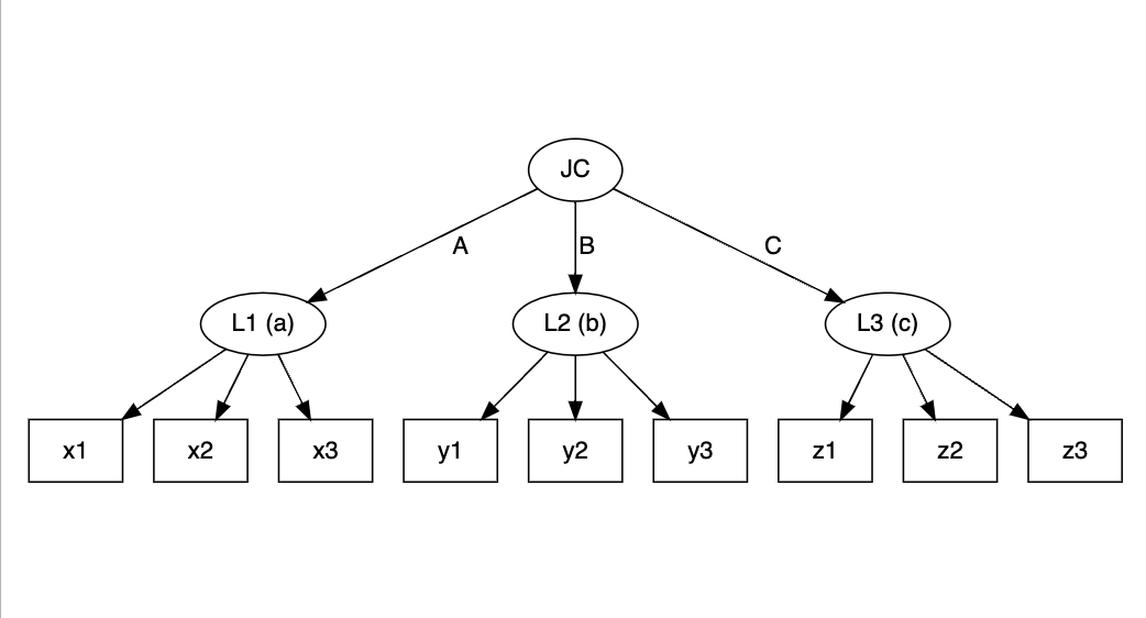
In some cases, you might need to define higher-level latent class
variables that are influenced by or comprise several other latent class
variables. For example, a higher-level variable P could be
a composite of L1, L2, and L3.
Here, note that you should define the number of latent classes for
P. This relationship can be represented as follows:
P[4] ~ L1 + L2 + L3
A critical aspect of model specification is ensuring measurement
invariance. This concept refers to the idea that the same latent
construct is being measured across different groups or time points. In
slca, you can assume measurement invariance by setting
constraints on your latent class variables. The constraints
argument is used to specify which latent class variables should be
measured in a homogeneous manner. This feature is crucial for
comparative studies where you need to ensure that the measurement
properties of your constructs are consistent across different sub-groups
or over time.
slca(L1[3] ~ x11 + x21 + x31,
     L2[3] ~ x12 + x22 + x32,
     L3[3] ~ x13 + x23 + x33,
     P[3] ~ L1 + L2 + L3,
     constraints = c("L1", "L2", "L3"))
If the model needs to be constrained for the transition probabilities
to be homogeneous, you can use ~ or -> to
represent the relationships you want to indicate, as follows:
slca(L1[3] ~ x11 + x21 + x31,
     L2[3] ~ x12 + x22 + x32,
     L3[3] ~ x13 + x23 + x33,
constraints = c("L1 ~ L2", "L2 -> L3"))library(slca)
lta <- slca(L1[3] ~ x1 + y1 + z1, L2[3] ~ x2 + y2 + z2, L3[3] ~ x3 + y3 + z3,
L1 ~ L2, L2 ~ L3, constraints = c("L1", "L2", "L3"))
plot(lta)
jlca <- slca(L1[3] ~ x1 + x2 + x3, L2[3] ~ y1 + y2 + y3, L3[3] ~ z1 + z2 + z3,
             JC[3] ~ L1 + L2 + L3)
plot(jlca)
lcamg <- slca(L1[3] ~ x1 + x2 + x3, L2[3] ~ y1 + y2 + y3, L3[3] ~ z1 + z2 + z3,
              JC[3] ~ L1 + L2 + L3, LG[3] ~ g1 + g2 + g3,
              LG ~ JC)
plot(lcamg)